Lab 1: Introduction to R
CRD 150 - Quantitative Methods in Community Research
Professor Noli Brazil
April 2, 2025
In this guide you will learn the basic fundamentals of the statistical software program R. Because R is not a prerequisite for the class, this guide assumes no background in the language. The objectives of the guide are as follows:
- Download R and RStudio
- Get familiar with the RStudio interface
- Understand R data types
- Understand R data structures, in particular vectors and data frames
- Understand R functions
- Understand R Markdown and the process for submitting assignments
This lab guide follows closely and supplements the material presented in Chapters 2, 4, and 20 in the textbook R for Data Science (RDS).
Assignment 1 is due by 12:00 pm, April 9th on Canvas.
See here for
assignment guidelines. You must submit an .Rmd file and its
associated .html file. Name the files:
yourLastName_firstInitial_asgn01. For example: brazil_n_asgn01
A note on lab guides
Lab guides are self-contained and self-guided. The expectation for each guide is to get through all of it either on your own or collaboratively. You do not need to turn in lab guides. However, it is important that you do not skip guides as lab material builds on one another.
What is R?
R is a free, open source statistical programming language. It is useful for data cleaning, analysis, and visualization. R is an interpreted language, not a compiled one. This means that you type something into R and it does it. It is both a command line software and a programming environment. It is an extensible, open-source language and computing environment for Windows, Macintosh, UNIX, and Linux platforms, which allows for the user to freely distribute, study, change, and improve the software.
Getting R
R can be downloaded from one of the “CRAN” (Comprehensive R Archive Network) sites. In the US, the main site is at https://cran.r-project.org/. Look in the “Download and Install R” area. Click on the appropriate link based on your operating system.
If you already have R on your computer, make sure you have the most updated version of R on your personal computer (4.4.3 “Trophy Case”).
Mac OS X
On the “R for macOS” page, there are multiple packages that could be downloaded. If you have a Mac with Apple Silicon, click on R-4.4.3-arm64.pkg; if you don’t have Silicon and are running on macOS 11 (Big Sur) or higher, click on R-4.4.3-x86_64.pkg; if you are running an earlier version of OS X, download the appropriate version listed under “Binaries for legacy macOS/OS X systems.”
After the package finishes downloading, locate the installer on your hard drive, double-click on the installer package, and after a few screens, select a destination for the installation of the R framework (the program) and the R.app GUI. Note that you will have to supply your computer’s Administrator’s password. Close the window when the installation is done.
An application will appear in the Applications folder: R.app.
Browse to the XQuartz download page. Click on the most recent version of XQuartz to download the application.
Run the XQuartz installer. XQuartz is needed to create windows to display many types of R graphics: this used to be included in MacOS until version 10.8 but now must be downloaded separately.
Windows
On the “R for Windows” page, click on the “base” link, which should take you to the “R-4.4.3 for Windows” page
On this page, click “Download R 4.4.3 for Windows”, and save the exe file to your hard disk when prompted. Saving to the desktop is fine.
To begin the installation, double-click on the downloaded file. Don’t be alarmed if you get unknown publisher type warnings. Window’s User Account Control will also worry about an unidentified program wanting access to your computer. Click on “Run” or “Yes”.
Select the proposed options in each part of the install dialog. When the “Select Components” screen appears, just accept the standard choices (the default). For Startup options, keep the default.
Note: Depending on the age of your computer and version of Windows, you may be running either a “32-bit” or “64-bit” version of the Windows operating system. If you have the 64-bit version (most likely), R will install the appropriate version (R x64 3.5.2) and will also (for backwards compatibility) install the 32-bit version (R i386 3.5.2). You can run either, but you will probably just want to run the 64-bit version.
What is RStudio?
If you click on the R program you just downloaded, you will find a very basic user interface. For example, below is what I get on a Mac
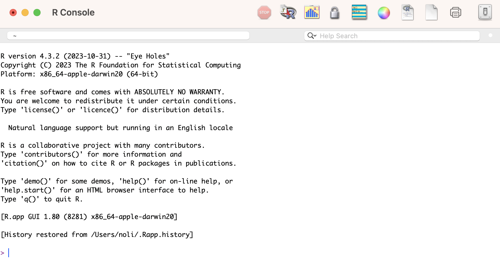
We will not use R’s direct interface to run analyses. Instead, we will use the program RStudio. RStudio gives you a true integrated development environment (IDE), where you can write code in a window, see results in other windows, see locations of files, see objects you’ve created, and so on. To clarify which is which: R is the name of the programming language itself and RStudio is a convenient interface.
Getting RStudio
To download and install RStudio, follow the directions below
- Navigate to RStudio’s download site
- Click on the “Download RStudio Desktop” link under the header “2: Install RStudio”. This will prompt you to save an installer package on your drive.
- Click on the installer that you downloaded. Follow the installation wizard’s directions, making sure to keep all defaults intact. After installation, RStudio should pop up in your Applications or Programs folder/menu.
Note that the most recent version of RStudio works only for certain operating systems (OS). If you have an older OS, you will need to download an older version RStudio, which you can find here.
The RStudio Interface
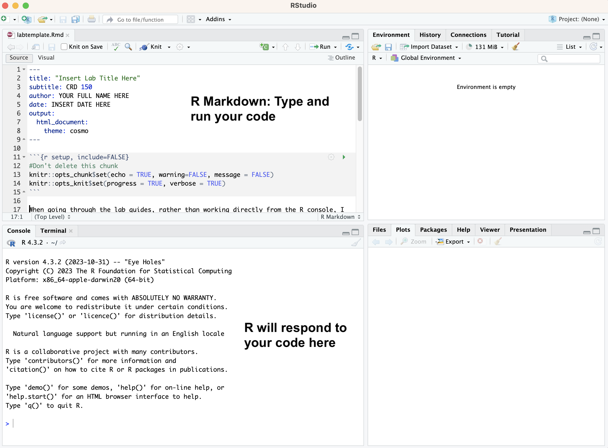
Open up RStudio. It may ask you to connect to R, which you’ve already downloaded. You should see the interface shown in the figure below which has three windows.
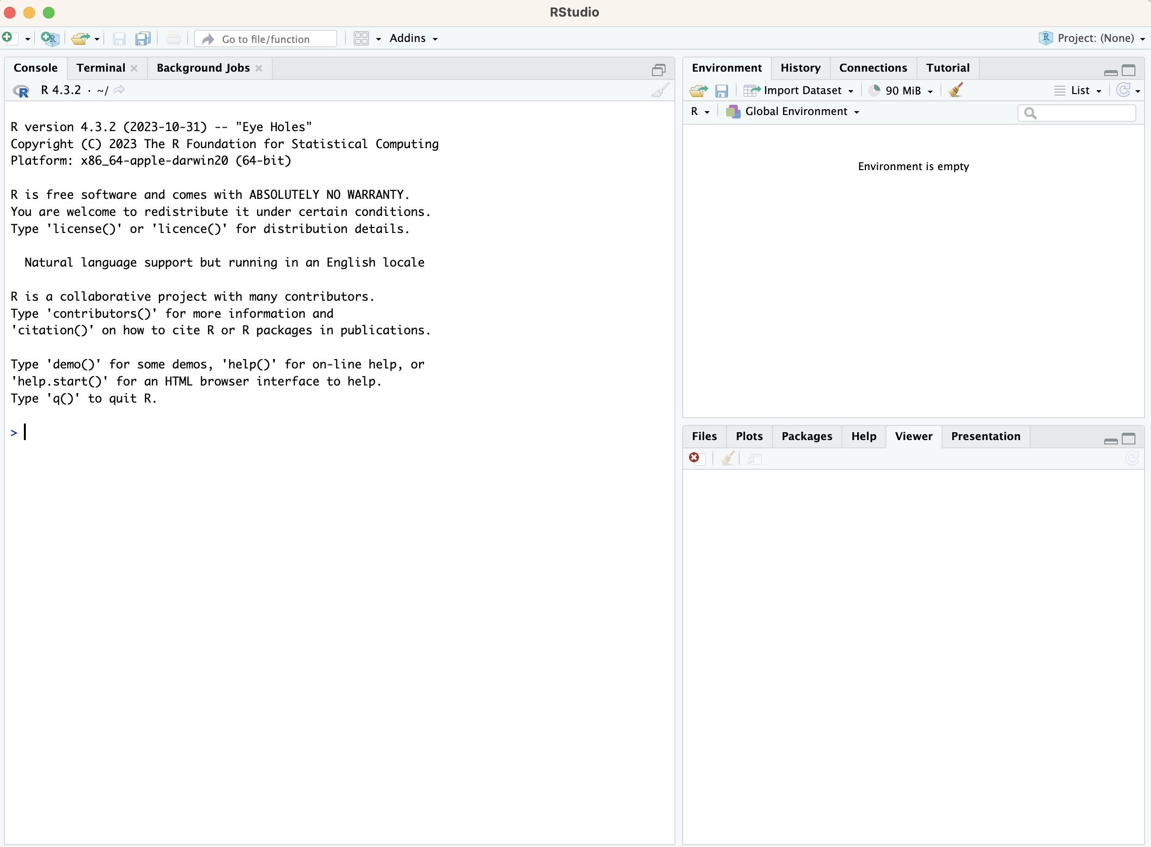
- Console (left) - The way R works is you write a
line of code to execute some kind of task on a data object. The R
Console allows you to run code interactively. The screen prompt
>is an invitation from R to enter its world. This is where you type code in, press enter to execute the code, and see the results. - Environment, History, and Connections tabs
(upper-right)
- Environment - shows all the R objects that are
currently open in your workspace. This is the place, for example, where
you will see any data you’ve loaded into R. When you exit RStudio, R
will clear all objects in this window. You can also click on
 to clear out all the objects loaded and created in your current
session.
to clear out all the objects loaded and created in your current
session. - History - shows a list of executed commands in the current session.
- Connections - you can connect to a variety of data
sources, and explore the objects and data inside the connection. I
typically don’t use this window, but you can.
- Tutorial - used to run tutorials that will help you
learn and master the R programming language.
- Environment - shows all the R objects that are
currently open in your workspace. This is the place, for example, where
you will see any data you’ve loaded into R. When you exit RStudio, R
will clear all objects in this window. You can also click on
- Files, Plots, Packages, Help and Viewer tabs
(lower-right)
- Files - shows all the files and folders in your current working directory (more on what this means later).
- Plots - shows any charts, graphs, maps and plots
you’ve successfully executed (we’ll be using this window starting in Lab
5).
- Packages - tells you all the R packages that you have access to (more on this in Lab 2).
- Help - shows help documentation for R commands that
you’ve called up.
- Viewer - allows you to view local web content (won’t be using this much).
- Presentation - used to display HTML slides.
There is actually fourth window. But, we’ll get to this window a little later (if you read the assignment guidelines you already know what this fourth window is).
For more information on each tab, check this resource.
Setting RStudio Defaults
While not required, I strongly suggest that you change preferences in RStudio to never save the workspace so you always open with a clean environment. See Ch. 8.1 of R4DS for some more background
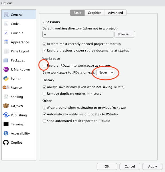
- From the Tools menu on RStudio, select Global Options.
- If not already highlighted, click on the General button from the left panel.
- Uncheck the following Restore box
- Restore .RData into workspace at startup
- Set Save Workspace to .RData on exit to Never.
- Click OK at the bottom to save the changes and close the preferences window. You may need to restart RStudio.
The reason for making these changes is that it is preferable for reproducibility to start each R session with a clean environment. You can restore a previous environment either by rerunning code or by manually loading a previously saved session.
The R Studio environment is modified when you execute code from files or from the console. If you always start fresh, you do not need to be concerned about things not working because of something you typed in the console, but did not save in a file.
You only need to set these preferences once.
R Data Types
Let’s now explore what R can do. R is really just a big fancy
calculator. For example, type in the following mathematical expression
next to the > in the R console (left window)
1+1Note that spacing does not matter: 1+1 will generate the
same answer as 1 + 1. Can you say hello to the
world?
hello world## Error in parse(text = input): <text>:1:7: unexpected symbol
## 1: hello world
## ^Nope. What is the problem here? We need to put quotes around it.
"hello world"## [1] "hello world"“hello world” is a character and R recognizes characters only if there are quotes around it. This brings us to the topic of basic data types in R. There are four basic data types in R: character, logical, numeric, and factors (there are two others - complex and raw - but we won’t cover them because they are rarely used).
Characters
Characters are used to represent words or letters in R. We saw this
above with “hello world”. Character values are also known as strings.
You might think that the value "1" is a number. Well, with
quotes around, it isn’t! Anything with quotes will be interpreted as a
character. No ifs, ands or buts about it.
Logicals
A logical takes on two values: FALSE or TRUE. Logicals are usually constructed with comparison operators, which we’ll go through more carefully in Lab 2. Think of a logical as the answer to a question like “Is this value greater than (lower than/equal to) this other value?” The answer will be either TRUE or FALSE. TRUE and FALSE are logical values in R. For example, typing in the following
3 > 2## [1] TRUEgives us a true. What about the following?
"prof visser" == "prof cannon"## [1] FALSENumeric
Numerics are separated into two types: integer and double. The
distinction between integers and doubles is usually not important. R
treats numerics as doubles by default because it is a less restrictive
data type. You can do any mathematical operation on numeric values. We
added one and one above. We can also multiply using the *
operator
2*3## [1] 6Divide
4/2## [1] 2And even take the logarithm!
log(1)## [1] 0log(0)## [1] -InfUh oh. What is -Inf? Well, you can’t take the logarithm
of 0, so R is telling you that you’re getting a non numeric value in
return. The value -Inf is another type of value type that
you can get in R. We’ll go through this and other weirdo values in Lab
2.
Factors
Think of a factor as a categorical variable. It is sort of like a character, but not really. It is actually a numeric code with character-valued levels. Think of a character as a true string and a factor as a set of categories represented as characters. We won’t use factors too much in this course.
R Data Structures
You learned that R has four basic data types. Now, let’s go through how
we can store data in R. That is, you type in the character “hello world”
or the number 3, and you want to store these values. You do this by
using R’s various data structures.
Vectors
A vector is the most common and basic R data structure and is pretty
much the workhorse of the language. A vector is simply a sequence of
values which can be of any data type but all of the same type. There are
a number of ways to create a vector depending on the data type, but the
most common is to insert the data you want to save in a vector into the
command c(). For example, to save the values 4, 16 and 9 in
a vector type in
c(4, 16, 9)## [1] 4 16 9You can also have a vector of character values
c("jonathan", "anne", "clare")## [1] "jonathan" "anne" "clare"The above code does not actually “save” the values 4, 16, and 9 - it
just presents it on the screen in a vector. If you want to use these
values again without having to type out c(4, 16, 9), you
can save it in a data object. At the heart of almost everything you will
do (or ever likely to do) in R is the concept that everything in R is an
object. These objects can be almost anything, from a single number or
character string (like a word) to highly complex structures like the
output of a plot, a map, or a summary of your statistical analysis.
You assign data to an object using the arrow sign <-.
This will create an object in R’s memory that can be called back into
the command window at any time. For example, you can save “hello world”
to a vector called b by typing in
b <- "hello world"
b
## [1] "hello world"You can pronounce the above as “b becomes ‘hello world’”.
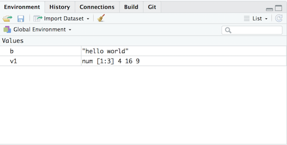
Similarly, you can save the numbers 4, 16 and 9 into a vector called v1
v1 <- c(4, 16, 9)
v1
## [1] 4 16 9You should see the objects b and v1 pop up in the Environment tab on the top right window of your RStudio interface.
Note that the name v1 is nothing special here. You could have named the object x or crd150 or your pet’s name (mine was charlie). You can’t, however, name objects using special characters (e.g. !, @, $) or only numbers (although you can combine numbers and letters, but a number cannot be at the beginning e.g. 2d2). For example, you’ll get an error if you save the vector c(4,16,9) to an object with the following names
123 <- c(4, 16, 9)
!!! <- c(4, 16, 9)
## Error in parse(text = input): <text>:2:5: unexpected assignment
## 1: 123 <- c(4, 16, 9)
## 2: !!! <-
## ^Also note that to distinguish a character value from a variable name, it needs to be quoted. “v1” is a character value whereas v1 is a variable. One of the most common mistakes for beginners is to forget the quotes.
brazil## Error: object 'brazil' not foundThe error occurs because R tries to print the value of the object
brazil, but there is no such object. So remember that any time
you get the error message object 'something' not found, the
most likely reason is that you forgot to quote a character value. If
not, it probably means that you have misspelled, or not yet created, the
object that you are referring to. I’ve included the common pitfalls and
R tips in this class resource.
Every vector has two key properties: type and
length. The type property indicates the data type that the
vector is holding. Use the command typeof() to determine
the type
typeof(b)## [1] "character"typeof(v1)## [1] "double"Note that a vector cannot hold values of different types. If
different data types exist, R will coerce the values into the highest
type based on its internal hierarchy: logical < integer < double
< character. Type in test <- c("r", 6, TRUE) in your
R console. What is the vector type of test?
The command length() determines the number of data
values that the vector is storing
length(b)## [1] 1length(v1)## [1] 3You can also directly determine if a vector is of a specific data
type by using the command is.X() where you replace
X with the data type. For example, to find out if
v1 is numeric, type in
is.numeric(b)## [1] FALSEis.numeric(v1)## [1] TRUEThere is also is.logical(), is.character(),
and is.factor(). You can also coerce a vector of one data
type to another. For example, save the value “1” and “2” (both in
quotes) into a vector named x1
x1 <- c("1", "2")
typeof(x1)
## [1] "character"To convert x1 into a numeric, use the command
as.numeric()
x2 <- as.numeric(x1)
typeof(x2)
## [1] "double"There is also as.logical(), as.character(),
and as.factor().
An important practice you should adopt early is to keep only
necessary objects in your current R Environment. For example, we will
not be using x2 any longer in this guide. To remove this object
from R forever, use the command rm()
rm(x2)The data frame object x2 should have disappeared from the Environment tab. Bye bye!
Also note that when you close down R Studio, the objects you created above will disappear for good. Unless you save them onto your hard drive (we’ll touch on saving data in Lab 2), all data objects you create in your current R session will go bye bye when you exit the program.
Data Frames
We learned that data values can be stored in data structures known as vectors. The next step is to learn how to store vectors into an even higher level data structure. The data frame can do this. Data frames store vectors of the same length. Create a vector called v2 storing the values 5, 12, and 25
v2 <- c(5,12,25)We can create a data frame using the command
data.frame() storing the vectors v1 and
v2 as columns
data.frame(v1, v2)## v1 v2
## 1 4 5
## 2 16 12
## 3 9 25Store this data frame in an object called df1
df1<-data.frame(v1, v2)df1 should pop up in your Environment window. You’ll notice
a  next to df1. This tells you that df1 possesses or
holds more than one object. Click on
and you’ll see the two vectors we saved into df1. Another neat
thing you can do is directly click on df1 from the Environment
window to bring up an Excel style worksheet on the top left window of
your RStudio interface. You can also type in
next to df1. This tells you that df1 possesses or
holds more than one object. Click on
and you’ll see the two vectors we saved into df1. Another neat
thing you can do is directly click on df1 from the Environment
window to bring up an Excel style worksheet on the top left window of
your RStudio interface. You can also type in
View(df1)to bring the worksheet up. You can’t edit this worksheet directly, but it allows you to see the values that a higher level R data object contains.
We can store different types of vectors in a data frame. For example, we can save the numeric vector v1 with a character vector v3.
v3 <- c("jonathan", "anne", "clare")
df2 <- data.frame(v1, v3)
df2
For higher level data structures like a data frame, use the function
class() to figure out what kind of object you’re working
with.
class(df2)## [1] "data.frame"We can’t use length() on a data frame because it has
more than one vector. Instead, it has dimensions - the number
of rows and columns. You can find the number of rows in a data frame
using nrow()
nrow(df1)## [1] 3Number of columns using ncol(df2)
ncol(df1)## [1] 2and the number of row and columns by using the command
dim()
dim(df1)## [1] 3 2Here, the data frame df1 has 3 rows and 2 columns. Data frames also have column names, which are characters.
colnames(df1)## [1] "v1" "v2"In this case, the data frame used the vector names for the column names.
We can extract columns from data frames by referring to their names
using the $ sign.
df1$v1## [1] 4 16 9We can also extract data from data frames using brackets
[ , ]
df1[,1]## [1] 4 16 9The value before the comma indicates the row, which you leave empty if you are not selecting by row. The value after the comma indicates the column, which you leave empty if you are not selecting by column. The above line of code selected the first column. Let’s select the 2nd row.
df1[2,]## v1 v2
## 2 16 12What is the value in the 2nd row and 1st column?
df1[2,1]## [1] 16We’ve been talking about the values in vectors and data frames rather abstractly. In practice, values, vectors and data frames have specific meaning in the context of data analysis. Let’s make things concrete. Take a look at this website showing crimes in California cities in 2016. Sacramento had 3,549 violent crime incidences. This is a data value (numeric!). The collection of violent crime counts for each city is a vector. The data frame has California cities as rows and the population, violent crime, homicide, and so on as columns. You learned about these elements in Handout 1. Now you see them in action in the R environment.
Functions
Let’s take a step back and talk about functions (also known as
commands). An R function is a packaged recipe that converts one or more
inputs (called arguments) into a single output. You execute most of your
tasks in R using functions. We have already used a couple of functions
above including typeof() and colnames(). Every
function in R will have the following basic format
functionName(arg1 = val1, arg2 = val2, ...)
In R, you type in the function’s name and set a number of options or parameters within parentheses that are separated by commas. Some options need to be set by the user - i.e. the function will spit out an error because a required option is blank - whereas others can be set but are not required because there is a default value established.
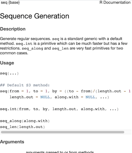
Let’s use the function seq() which makes regular
sequences of numbers. You can find out what a function does and its
options by calling up its help documentation by typing ?
and the function name. The documentation should also provide some
examples of the function at the bottom of the page.
? seqThe help documentation should have popped up in the bottom right
window of your RStudio interface. The function contains
from, to, by, and other
arguments. Under the Arguments section you can find what each of these
parameters means.
The description of the arguments from and
to are the starting and (maximal) end values of the
sequence. Of length 1 unless just from is supplied as an unnamed
argument. Type the arguments from = 1, to = 10 inside
the parentheses of seq()
seq(from = 1, to = 10)## [1] 1 2 3 4 5 6 7 8 9 10You should get the same result if you type in
seq(1, 10)## [1] 1 2 3 4 5 6 7 8 9 10The code above demonstrates something about how R resolves function
arguments. When you use a function, you can always specify all the
arguments in arg = value form. But if you do not, R
attempts to resolve by position. So in the code seq(1, 10),
it is assumed that we want a sequence from = 1 that goes
to = 10 because we typed 1 before 10. Type in 10 before 1
and see what happens.
Each argument requires a certain type of data type. For example,
you’ll get an error when you use a character in seq()
seq("p", "w")## Error in seq.default("p", "w"): 'from' must be a finite numberAlthough the lab guides and course textbooks should get you through a lot of the functions that are needed to successfully accomplish tasks for this class, you will need to rely on the help documentation to better understand how functions work. There are also a number of useful online resources on R and RStudio that you can look into if you get stuck or want to learn more. We outline these resources here. If you ever get stuck, check this resource out first to troubleshoot before immediately asking a friend or the instructor/TA.
R Scripting
In running the few lines of code above, we’ve asked you to work
directly in the R Console and issue commands in an interactive
way. That is, you type a command after >, you hit
enter/return, R responds, you type the next command, hit enter/return, R
responds, and so on. As described in Handout 1, instead of writing the
command directly into the console, you should write it in a script. The
process is now: Type your command in the script. Run the code from the
script. R responds. You get results. You can write two commands in a
script. Run both simultaneously. R responds. You get results. This is
the basic flow. In your homework assignments, we will be asking you to
submit code in an R Markdown file. R Markdown allows you to create
documents that serve as a neat record of your analysis. Think of it as a
word document, but instead of sentences in an essay, you are writing
code for a data analysis.
Rather than copying and pasting code from the lab guides into the R Console as you’ve been doing up to this point, type it into an R Markdown file and then run the code from there. Even though you do not need to turn in the labs, running the lab code in your own R Markdown file will give you practice for your assignments. Plus, the code is in your document, so you can add explanatory text or supplement the guide’s code with your own code.
Just like for each assignment, I will provide an R Markdown template for each lab. Download the R Markdown Lab template into an appropriate folder on your hard drive. It’s best to set up on your hard drive a clean and efficient file management structure for this class as described in the assignment guidelines. For example, below is where I would save Lab 1’s R Markdown file on my Mac laptop (I named the file “Lab 1”).
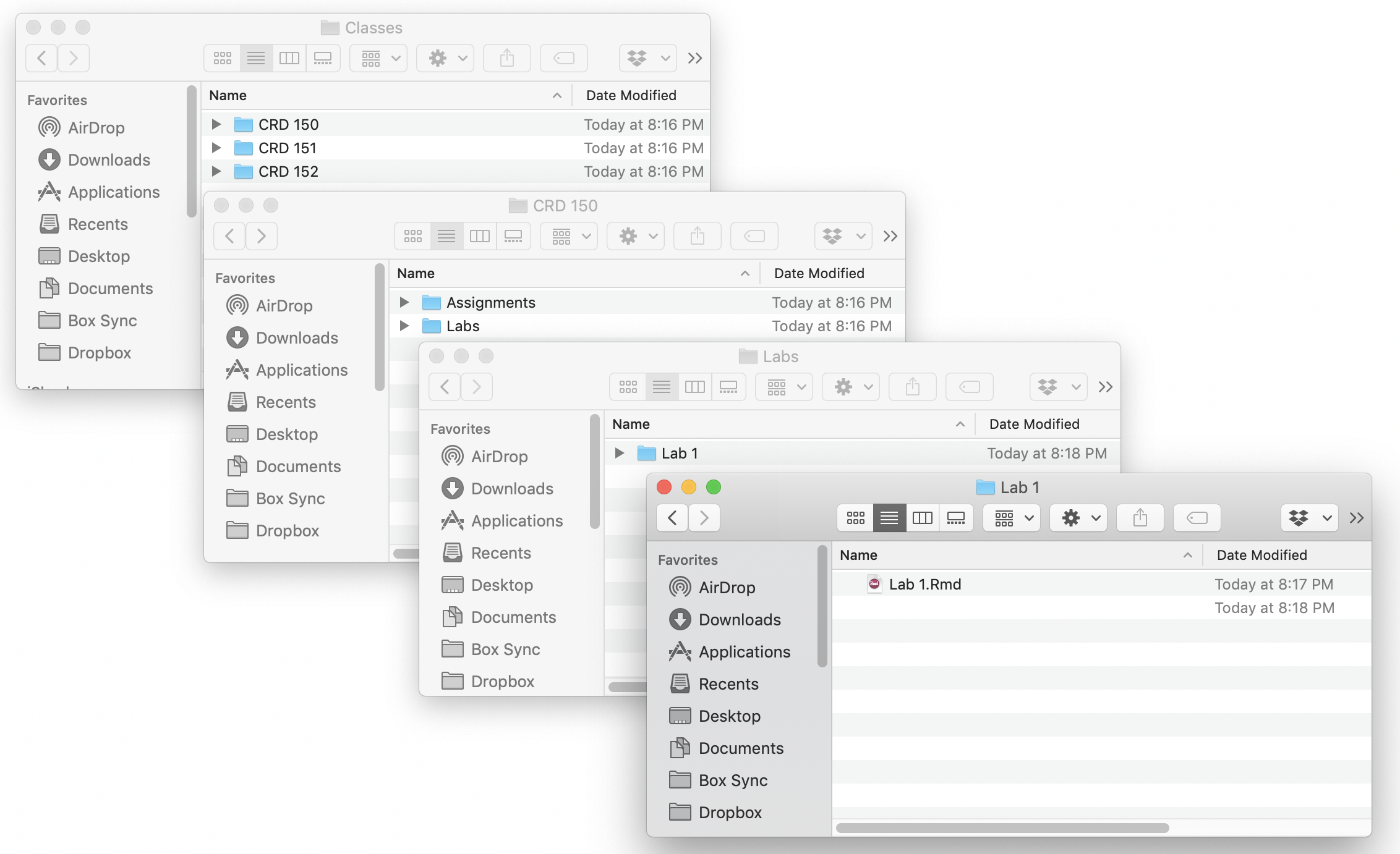
When you knit this RMarkdown, the resulting html file will be located in this folder.
Open the file in R Studio by clicking on File from the top menu, click on Open File, navigate to your Lab 1 folder, and click on the Lab 1 R Markdown file you downloaded. Once you do this, if there isn’t already one on your console, a fourth window should pop up in the top left showing you an R Markdown file.
In this file, change the title to “Lab 1” and insert your name and
date. Don’t change anything else inside the YAML (the stuff at the top
in between the ---). Also don’t change the following
chunk.
```{r setup, include=FALSE}
knitr::opts_chunk$set(echo = TRUE, warning=FALSE, message = FALSE)
```
All your code should go inside areas designated as
```{r}
#Type your code here
```
For example, you would write the code 1+1 as
```{r}
1+1
```
From the file, run the code. R responds. You get results.
Now is a good time to read through the class assignment guidelines as they go through the basics of R Markdown files. Go through this guide carefully as you will need to submit all your homework assignments using R Markdown.

This
work is licensed under a
Creative
Commons Attribution-NonCommercial 4.0 International License.
Website created and maintained by Noli Brazil