Lab 2: Data Wrangling
CRD 150 - Quantitative Methods in Community Research
Professor Noli Brazil
April 9, 2025
In this guide you will learn how to download, clean and manage data - a process known as Data Wrangling - in R. You will be working with data on California counties. The objectives of this guide are as follows
- Learn how to read data into R
- Learn about tidyverse
- Learn data wrangling functions
This lab guide follows and supplements the material presented in Chapters 4 and 8-13 in the textbook R for Data Science (RDS) and the class Handout 2.
Assignment 2 is due by 12:00 pm, April 16 on Canvas.
See here for
assignment guidelines. You must submit an .Rmd file and its
associated .html file. Name the files:
yourLastName_firstInitial_asgn02. For example: brazil_n_asgn02.
Open up a R Markdown file
Rather than working directly from the R console, I recommended typing
in lab code into an R Markdown and working from there. This will give
you more practice and experience working in the R Markdown environment,
which you will need to do for all of your assignments. Plus you can add
your own comments to the code to ensure that you’re understanding what
is being done. Download the lab
template into an appropriate folder on your hard drive (preferably,
a folder named ‘Lab 2’), open it in R Studio, and type and run your lab
code there. The template is also located on Canvas under Files. Change
the title (“Lab 2”) and insert your name and date. Don’t change anything
else inside the YAML (the stuff at the top in between the
---). Also keep the grey chunk after the YAML. For a
rundown on the use of R Markdown, see the assignment
guidelines.
R Packages
At the end of Lab 1 we learned
about R functions. Functions do not exist in a vacuum, but exist within
R packages. Packages
are the fundamental units of reproducible R code. They include R
functions, the documentation that describes how to use them, and sample
data. At the top left of a function’s help documentation, you’ll find in
curly brackets the R package that the function is housed in. For
example, type in your console ? seq. At the top left of the
help documentation, you’ll find that seq() is in the
package base. All the functions we have used so far are
part of packages that have been pre-installed and pre-loaded into R. For
all new packages, you need to install and load them.
In this lab and all labs from here on out, we will be using commands
from the package tidyverse. Tidyverse is a collection of
high-powered, consistent, and easy-to-use packages developed by a number
of thoughtful and talented R developers. In order to use functions in a
new package, you first need to install the package using the
install.packages() command.
install.packages("tidyverse")You should see a bunch of gobbledygook roll through your console screen. Don’t worry, that’s just R downloading all of the other packages and applications that tidyverse relies on. These are known as dependencies. Unless you get a message in red that indicates there is an error (like we saw in Lab 1 when we typed in hello world without quotes), you should be fine.
When you are installing a package, you may get the message that asks “Do you want to install from sources the packages which need compilation?” This often means that the package has updated recently on CRAN isn’t yet available for your operating system (which can take a day or two). In many cases, you can deal with this by updating R to its most recent version. If you already have the most recent version, the easiest thing to do is type in “no.” If you say no, you won’t get the most recent version of the package. But this might be just fine, unless you were specifically installing because of an update. If you say yes, the package will be built from source locally. If it has compiled code and you’ve never set up build tools for R, then this won’t actually succeed.
Next, you will need to load the package into your working
environment. You need to do this every time you start RStudio. We do
this using the library() function. Notice there are no
quotes around tidyverse this time.
library(tidyverse)The Packages window at the lower-right of your RStudio shows all the
packages you currently have installed. If you don’t have a package
listed in this window, you’ll need to use the
install.packages() function to install it. If the package
is checked, that means it is loaded into your current R session
For example, here is a section of my Packages window.
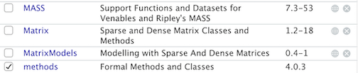
The only packages loaded into my current session is
methods, a package that is loaded every time you open
an R session. Let’s say we use install.packages() to
install the package matrixStats. The window now looks
like:
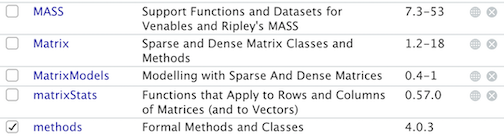
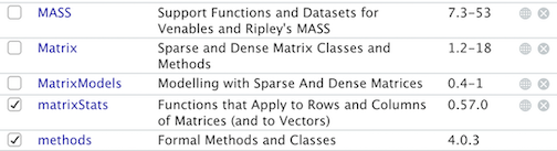
When you load it in using library(), a check mark
appears next to matrixStats.
Note that you only need to install packages once
(install.pacakges()), but you need to load them each time
you relaunch RStudio (library()). Repeat after me:
Install once, library every time. This means your R Markdown should
never have the function install.pacakges() but will likely
always have the function library().
Are you ready to enter the tidyverse? Yes, of course, so here is a badge! Wear it proudly my young friends! And away we go!

Reading data
One of the first steps in the Data Wrangling process is to read in
your dataset. Most of the data files you will encounter are
comma-delimited (or comma-separated) files, which have .csv
extensions. Comma-delimited means that columns are separated by commas.
I uploaded a file on Canvas (Files - Week 2 - Lab) containing the number
of Hispanic, white, Asian, and black residents in 2018 in California
counties taken from the United States American Community
Survey. Download the file week2data.csv and save it into
the same folder where your Lab 2 R Markdown file resides. The
data that you will analyze in your RMarkdown has to always be saved in
the same folder as your RMarkdown otherwise it will not knit.
The record layout/codebook for the file can be found here.
To read in the csv file, first make sure that R is pointed to the
folder you saved your data into. Type in getwd() to find
out the current directory
getwd()and setwd("directory name") to set the directory to the
folder containing the data, where “directory name” is the path to the
folder on your hard drive containing this lab’s data.
In my Mac OS computer, the file is located in the folder shown in the figure below. To get the Info window, right click on the file, and select “Get Info”.
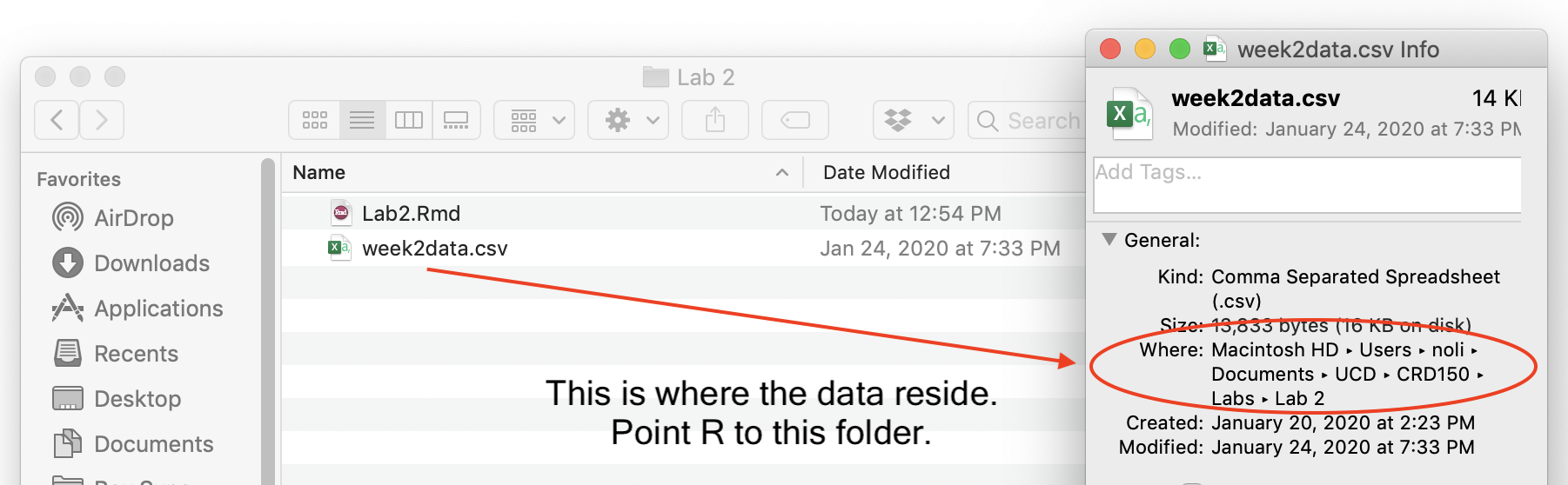
Using a Mac laptop, I type in the following command to set the directory to the folder containing my data.
setwd("~/Documents/UCD/CRD150/Labs/Lab 2")You can also copy the path from the Get Info window above, and paste
it within quotes in setwd().
For a Windows system, you can find the pathway of a file by right
clicking on it and selecting Properties. You will find that instead of a
forward slash like in a Mac, a Windows path will be indicated by a
single back slash \. R doesn’t like this because it thinks
of a single back slash as an escape
character. Use instead two back slashes \\
setwd("C:\\Users\\noli\\Desktop\\Classes\\CRD150\\Lab 2")or a forward slash /.
setwd("C:/Users/noli/Desktop/Classes/CRD150/Lab 2")You can also manually set the working directory by clicking on Session -> Set Working Directory -> Choose Directory on a Mac or Tools -> Change Working Directory on a Windows machine. Be careful to consider the side effects of changing your working directory, specifically relative file references in your code (for datasets, source files, etc) will become invalid when you change working directories. Because these side effects can cause confusion and errors, it’s usually best to start within the working directory associated with your project and remain there for the duration of your session.
Once you’ve set your directory, use the function
read_csv() and plug in the name of the file in quotes
inside the parentheses. Make sure you include the .csv
extension.
counties <- read_csv("week2data.csv")You should see the object counties pop up in your
Environment window (top right). First thing you should do when you bring
in a data set is to look at it to make sure you know what you have and
nothing went drastically wrong when reading in the data. One way to look
at the data is to print it on your screen. Do this using the
glimpse() command
glimpse(counties)## Rows: 58
## Columns: 8
## $ GEOID <chr> "06001", "06003", "06005", "06007", "06009", "06011", "06013", "…
## $ name <chr> "Alameda County", "Alpine County", "Amador County", "Butte Count…
## $ state <chr> "California", "California", "California", "California", "Califor…
## $ hisp <dbl> 367041, 117, 4943, 35445, 5166, 12539, 284003, 5281, 23279, 5094…
## $ asian <dbl> 468356, 8, 565, 9852, 527, 328, 177544, 741, 7805, 96128, 729, 3…
## $ black <dbl> 175063, 18, 764, 3282, 258, 186, 93140, 484, 1614, 45217, 212, 1…
## $ white <dbl> 524881, 777, 29571, 164184, 36932, 7800, 504818, 17233, 145153, …
## $ tpop <dbl> 1629615, 1203, 37306, 225207, 45057, 21479, 1123678, 27442, 1850…You get a quick, compact summary of your data The function takes one argument: the name of a data frame. It then tells us how many rows it has, how many variables there are, what these variables are called, and what kind of data are associated with each variable. This function is useful when we’re working with a data set containing many variables.
If you like viewing your data through an Excel style worksheet, type
in View(counties), and counties should pop up in
the top left window of your R Studio interface. Scroll up and down, left
and right. Take some time to understand the format of the data set. What
do the columns represent? Rows?
tidyverse can read in more than just .csv files. It
has a suite of read_ functions that are a part of the
subpackage readr. The goal of readr is
to provide a fast and friendly way to read rectangular data (like csv,
tsv, and fwf). It is designed to flexibly parse many types of data found
in the wild, while still cleanly failing when data unexpectedly changes.
To learn more about these functions, see readr’s
dedicated site.
By learning how to read in data, you’ve earned another tidyverse badge! Hooray!

Tibbles
The data set that you brought in above using read_csv()
saved the file in a special R object known as a tibble.
Although the tidyverse works with all data objects, its
fundamental object type is the tibble. Tibbles are essentially a special
variant of data frames that have desirable properties for printing and
joining. To illustrate comparisons between tibbles and regular data
frames, let’s bring in the county data we downloaded above but using the
function read.csv(), which will bring in files as regular
data frames.
counties.df <- read.csv("week2data.csv")The first difference between regular data frames and tibbles is how the dataset “looks.” First, the tibble.
counties## # A tibble: 58 × 8
## GEOID name state hisp asian black white tpop
## <chr> <chr> <chr> <dbl> <dbl> <dbl> <dbl> <dbl>
## 1 06001 Alameda County California 367041 468356 175063 524881 1629615
## 2 06003 Alpine County California 117 8 18 777 1203
## 3 06005 Amador County California 4943 565 764 29571 37306
## 4 06007 Butte County California 35445 9852 3282 164184 225207
## 5 06009 Calaveras County California 5166 527 258 36932 45057
## 6 06011 Colusa County California 12539 328 186 7800 21479
## 7 06013 Contra Costa County California 284003 177544 93140 504818 1123678
## 8 06015 Del Norte County California 5281 741 484 17233 27442
## 9 06017 El Dorado County California 23279 7805 1614 145153 185015
## 10 06019 Fresno County California 509442 96128 45217 293677 971616
## # ℹ 48 more rowsTibbles have a refined print method that shows only the first 10 rows, and only the columns that fit on the screen. In addition, each column reports its name and type.
Tibbles are designed so that you don’t accidentally overwhelm your console when you print large data frames. Compare the print output above to what you get with a data frame
counties.dfUgly, right?
Not all functions work with tibbles, particularly those that are specific to spatial data. As such, we’ll be using a combination of tibbles and regular data frames throughout the class, with a preference towards tibbles where possible.
Note that when you search on Google for how to do something in R, you
will likely get non tidyverse ways of doing things. Most of these
suggestions are fine, but some are not and may screw you up down the
road. For example, always use read_csv() to read in data.
Do not use read.csv(). My advice is to try to stick with
tidyverse functions to do things in R. This is why our textbook RDS is a
valuable resource.
Anyway, you earned another badge. Yes!

Data Wrangling
It is rare that the data you download are in exactly the right form for analysis. For example, rather than all counties in the tibble counties, you might want to analyze just Northern California counties. Or you might want to discard certain variables from the dataset to reduce clutter.
In this lab, we won’t have time to go through all of the methods and functions in R that are associated with the data wrangling process. We will cover more in Lab 3 and later labs. Many methods you will have to learn on your own given the specific tasks you will need to accomplish. In the rest of this guide, we’ll go through some of the basic data wrangling techniques using the functions found in the package dplyr, which was automatically installed and loaded when you brought in the tidyverse package.
Selecting variables
In practice, most of the data files you will download will contain
variables you won’t need. It is easier to work with a smaller dataset as
it reduces clutter and clears up memory space, which is important if you
are executing complex tasks on a large number of observations. Use the
command select() to keep variables by name. Visually, we
are doing this (taken from the RStudio cheatsheet)
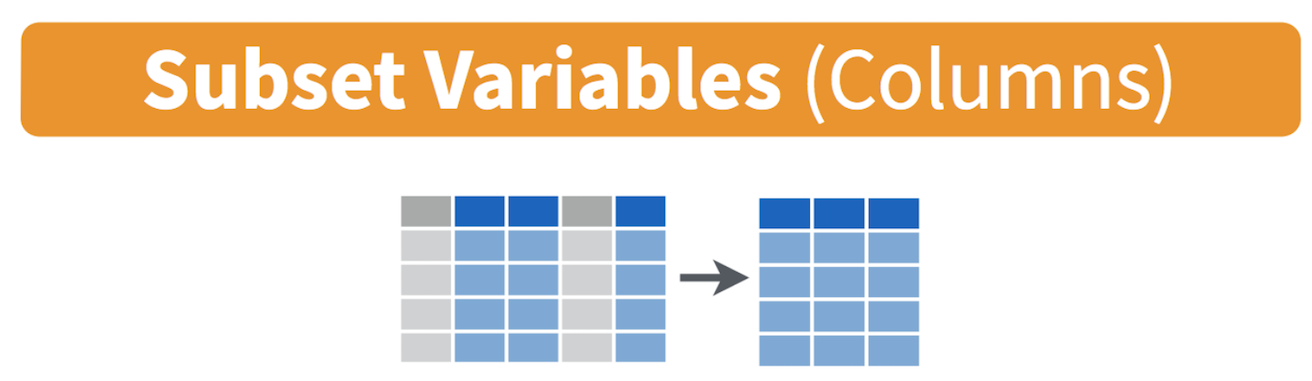
To see the names of variables in the dataset counties, use
the names() command.
names(counties)## [1] "GEOID" "name" "state" "hisp" "asian" "black" "white" "tpop"Let’s keep GEOID, name, hisp, asian, black, white, and tpop
select(counties, GEOID, name, hisp, asian, black, white, tpop)## # A tibble: 58 × 7
## GEOID name hisp asian black white tpop
## <chr> <chr> <dbl> <dbl> <dbl> <dbl> <dbl>
## 1 06001 Alameda County 367041 468356 175063 524881 1629615
## 2 06003 Alpine County 117 8 18 777 1203
## 3 06005 Amador County 4943 565 764 29571 37306
## 4 06007 Butte County 35445 9852 3282 164184 225207
## 5 06009 Calaveras County 5166 527 258 36932 45057
## 6 06011 Colusa County 12539 328 186 7800 21479
## 7 06013 Contra Costa County 284003 177544 93140 504818 1123678
## 8 06015 Del Norte County 5281 741 484 17233 27442
## 9 06017 El Dorado County 23279 7805 1614 145153 185015
## 10 06019 Fresno County 509442 96128 45217 293677 971616
## # ℹ 48 more rowsA shortcut way of doing this is to use the :
operator.
select(counties, GEOID, name, hisp:tpop)## # A tibble: 58 × 7
## GEOID name hisp asian black white tpop
## <chr> <chr> <dbl> <dbl> <dbl> <dbl> <dbl>
## 1 06001 Alameda County 367041 468356 175063 524881 1629615
## 2 06003 Alpine County 117 8 18 777 1203
## 3 06005 Amador County 4943 565 764 29571 37306
## 4 06007 Butte County 35445 9852 3282 164184 225207
## 5 06009 Calaveras County 5166 527 258 36932 45057
## 6 06011 Colusa County 12539 328 186 7800 21479
## 7 06013 Contra Costa County 284003 177544 93140 504818 1123678
## 8 06015 Del Norte County 5281 741 484 17233 27442
## 9 06017 El Dorado County 23279 7805 1614 145153 185015
## 10 06019 Fresno County 509442 96128 45217 293677 971616
## # ℹ 48 more rowsThe : operator tells R to select all the variables from
hisp to tpop. This operator is useful when you’ve got
a lot of variables to keep and they all happen to be ordered
sequentially.
You can use the select() command to keep variables
except for the ones you designate. For example, to keep all
variables in counties except state type in
select(counties, -state)The negative sign tells R to exclude the variable named right after.
You can delete multiple variables. For example, if you wanted to keep
all variables except name and state, you would type in
select(counties, -name, -state).
Note that we didn’t save any of the above changes. To save them, you need to either replace the object with the changes, or create a new object with the changes. Let’s save this change back into a new tibble called counties1. You should see counties1 pop up in your Environment window.
counties1 <- select(counties, -state)Creating new variables
The mutate() function allows you to create new variables
within your dataset. This is important when you need to transform
variables in some way - for example, calculating a ratio or adding two
variables together. Visually, you are doing this
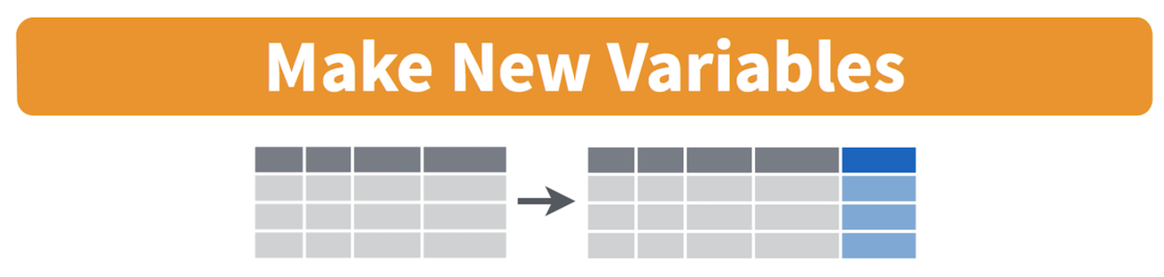
You can use the mutate() command to generate as many new
variables as you would like. For example, let’s construct five new
variables in counties1: the proportion of residents who are
non-Hispanic white, non-Hispanic Asian, non-Hispanic black, and
Hispanic. Name these variables pwhite, pasian,
pblack, and phisp, respectively.
mutate(counties1, pwhite = white/tpop, pasian = asian/tpop,
              pblack = black/tpop, phisp = hisp/tpop)
Note that you can create new variables based on the variables you
just created in the same line of code (Wow!). For example, you can
create a variable named diff that represents the difference
between the percent non-Hispanic white and percent non-Hispanic black
after creating both variables within the same mutate()
command. Let’s save these changes back into counties1
counties1 <- mutate(counties1, pwhite = white/tpop, pasian = asian/tpop,
              pblack = black/tpop, phisp = hisp/tpop,
              diff = pwhite-phisp)
View counties1 to verify that you’ve successfully created these variables.
glimpse(counties1)Filtering
Filtering means selecting rows/observations based on their values. To
filter in R, use the command filter(). Visually, filtering
rows looks like this.
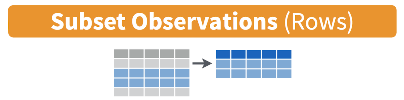
The first argument in the parentheses of this command is the name of
the data frame. The second and any subsequent arguments (separated by
commas) are the expressions that filter the data frame. For example, we
can keep just Sacramento county from counties1 using its FIPS
code, which is the county’s unique ID (note that we’re not saving
this change since we are not using the assignment operator
<-).
filter(counties1, GEOID == "06067")The double equal operator == means equal to. The command
is telling R to keep the rows in counties1 whose GEOID
equals “06067”. There are quotes around 06067 because GEOID is
a character
variable.
We can also explicitly exclude cases and keep everything else by
using the not equal operator !=. The following code
excludes Sacramento county.
filter(counties1, GEOID != "06067")What about filtering if a county has a value greater than a specified value? For example, counties with a proportion Hispanic greater than 0.5 (50%).
filter(counties1, phisp > 0.50)What about less than 0.5 (50%)?
filter(counties1, phisp < 0.50)Both lines of code do not include counties that have a proportion
Hispanic equal to 0.5. We include it by using the less than or equal
operator <= or greater than or equal operator
>=.
filter(counties1, phisp <= 0.5)In addition to comparison operators, filtering may also utilize
logical operators that make multiple selections. There are three basic
logical operators: & (and), | (or), and
! (not). We can keep counties with phisp greater
than 0.5 and pasian greater than 0.05 by using
&.
filter(counties1, phisp > 0.50 & pasian > 0.05)Use | to keep counties with a GEOID of “06067”
(Sacramento) or “06113” (Yolo)
filter(counties1, GEOID == "06067" | GEOID == "06113")Arrange
We use the arrange() function to sort a data frame by
one or more variables. You might want to do this to get a sense of which
cases have the highest or lowest values in your data set or sort
counties by their name. For example, let’s sort in ascending order
counties by proportion Hispanic.
arrange(counties1, phisp)## # A tibble: 58 × 12
## GEOID name hisp asian black white tpop pwhite pasian pblack phisp
## <chr> <chr> <dbl> <dbl> <dbl> <dbl> <dbl> <dbl> <dbl> <dbl> <dbl>
## 1 06105 Trinity … 937 141 104 10796 13037 0.828 0.0108 0.00798 0.0719
## 2 06063 Plumas C… 1599 148 160 15640 18724 0.835 0.00790 0.00855 0.0854
## 3 06057 Nevada C… 9109 1090 541 84389 98838 0.854 0.0110 0.00547 0.0922
## 4 06089 Shasta C… 17218 5195 1951 143919 178919 0.804 0.0290 0.0109 0.0962
## 5 06003 Alpine C… 117 8 18 777 1203 0.646 0.00665 0.0150 0.0973
## 6 06091 Sierra C… 290 0 4 2509 2885 0.870 0 0.00139 0.101
## 7 06043 Mariposa… 1870 168 215 14309 17658 0.810 0.00951 0.0122 0.106
## 8 06023 Humboldt… 14986 3886 1389 101460 135490 0.749 0.0287 0.0103 0.111
## 9 06009 Calavera… 5166 527 258 36932 45057 0.820 0.0117 0.00573 0.115
## 10 06109 Tuolumne… 6385 593 924 43565 53899 0.808 0.0110 0.0171 0.118
## # ℹ 48 more rows
## # ℹ 1 more variable: diff <dbl>Trinity county has the lowest percent Hispanic with 7.19.
By default, arrange() sorts in ascending order. We can
sort by a variable in descending order by using the desc()
function on the variable we want to sort by. For example, to sort
counties1 by phisp in descending order we use
arrange(counties1, desc(phisp))## # A tibble: 58 × 12
## GEOID name hisp asian black white tpop pwhite pasian pblack phisp
## <chr> <chr> <dbl> <dbl> <dbl> <dbl> <dbl> <dbl> <dbl> <dbl> <dbl>
## 1 06025 Imperia… 1.50e5 2263 4109 20372 1.80e5 0.113 0.0126 0.0228 0.834
## 2 06107 Tulare … 2.92e5 14622 5973 135372 4.59e5 0.295 0.0319 0.0130 0.636
## 3 06069 San Ben… 3.46e4 1564 437 20872 5.87e4 0.356 0.0267 0.00745 0.589
## 4 06011 Colusa … 1.25e4 328 186 7800 2.15e4 0.363 0.0153 0.00866 0.584
## 5 06047 Merced … 1.56e5 19593 8007 77092 2.67e5 0.288 0.0733 0.0299 0.582
## 6 06053 Montere… 2.51e5 24213 10621 132600 4.33e5 0.306 0.0559 0.0245 0.579
## 7 06039 Madera … 8.79e4 3035 4753 54145 1.54e5 0.351 0.0197 0.0308 0.569
## 8 06031 Kings C… 8.07e4 5463 8916 49728 1.50e5 0.331 0.0364 0.0594 0.537
## 9 06019 Fresno … 5.09e5 96128 45217 293677 9.72e5 0.302 0.0989 0.0465 0.524
## 10 06071 San Ber… 1.11e6 142802 168985 632557 2.12e6 0.298 0.0673 0.0797 0.523
## # ℹ 48 more rows
## # ℹ 1 more variable: diff <dbl>Imperial county has the largest percent Hispanic with 83.4.
Pipes
One of the important innovations from the tidyverse is the pipe
operator %>%. You use the pipe operator when you want to
combine multiple operations into one continuous line of code. For
example, we can use a pipe to combine all the commands we executed on
the object counties from the sections Selecting
variables to Filtering in one continuous line of code.
counties2 <- counties %>%
            select(-state) %>%
            mutate(pwhite = white/tpop, pasian = asian/tpop,
                    pblack = black/tpop, phisp = hisp/tpop,
                    diff = pwhite-phisp) %>%
            filter(GEOID == "06067" | GEOID == "06113")
Let’s break down what the pipe is doing here. First, you start out
with your dataset counties. You “pipe” %>% that
into the command select(). Notice that you didn’t have to
type in counties inside the select() command -
%>% pipes that in for you. select() deletes
state and then pipes this result into the command
mutate() to create new variables. This tibble gets piped to
filter() to select just Sacramento and Yolo counties.
Finally, the code saves the result into a new tibble counties2
which we designated at the beginning with the arrow operator.
Piping makes code clearer, and simultaneously gets rid of the need to define any intermediate objects that you would have needed to keep track of while reading the code. PIPE, Pipe, and pipe whenever you can. Badge it!
Saving Data
Let’s save a dataset containing race/ethnicity for Sacramento and
Yolo counties. Use write_csv() to save the data frame or
tibble as a csv file in the folder of your current working
directory.
write_csv(counties2, "lab2_file.csv")The first argument is the name of the R object you want to save. The
second argument is the name of the csv file in quotes. Make sure to add
the .csv extension. The file is saved in the folder you set as the
current working directory (remember, use getwd() to
determine the current directory). You’re done! Time to
celebrate.

This
work is licensed under a
Creative
Commons Attribution-NonCommercial 4.0 International License.
Website created and maintained by Noli Brazil