Lab 5: Spatial Data in R
CRD 150 - Quantitative Methods in Community Research
Professor Noli Brazil
April 30, 2025
In this guide you will acquire the skills needed to process and present spatial data in R. The objectives of the guide are as follows
- Understand how spatial data are processed in R
- Learn basic data wrangling operations on spatial data
- Learn how to make a map in R
This lab guide follows closely and supplements the material presented in Chapters 1, 2.1, 2.2, 8 and 9 in the textbook Geocomputation with R (GWR) and class Handout 5.
Assignment 5 is due by 12:00 pm, May 7th on Canvas. See
here for
assignment guidelines. You must submit an .Rmd file and its
associated .html file. Name the files:
yourLastName_firstInitial_asgn05. For example: brazil_n_asgn05.
Open up a R Markdown file
Download the Lab
template into an appropriate folder on your hard drive (preferably,
a folder named ‘Lab 5’), open it in R Studio, and type and run your code
there. The template is also located on Canvas under Files. Change the
title (“Lab 5”) and insert your name and date. Don’t change anything
else inside the YAML (the stuff at the top in between the
---). Also keep the grey chunk after the YAML. For a
rundown on the use of R Markdown, see the assignment
guidelines
Installing and loading packages
You’ll need to install the following packages in R. You only need to
do this once, so if you’ve already installed these packages, skip the
code. Also, don’t put these install.packages() commands in
your R Markdown document. Copy and paste the code in the R Console.
We’ll talk about what functions these packages provide as they come up
in the guide.
install.packages("sf")
install.packages("tigris")
install.packages("tmap")
install.packages("RColorBrewer")You’ll need to load the following packages using
library(). Unlike installing, you will always need to load
packages whenever you start a new R session.
library(tidyverse)
library(tidycensus)
library(flextable)
library(sf)
library(tigris)
library(tmap)
library(RColorBrewer)Spatial data in R
The main package we will use for handling spatial data in R is the tidy friendly sf package. sf stands for simple features. What is a feature? A feature is thought of as a thing, or an object in the real world, such as a building or a tree. A county can be a feature. As can a city and a neighborhood. Features have a geometry describing where on Earth the features are located, and they have attributes, which describe other properties. Think back to Lab 3 - we were working with counties. The difference between what we were doing then and what we will be doing in this lab is that counties in Lab 3 had attributes (e.g. percent Hispanic, total population), but they did not have geometries. As such, we could not put them on a map because we didn’t have their specific geographic coordinates. This is what separates nonspatial and spatial data in R.
Bringing in spatial data
sf is the specific type of data object that deals with spatial information in R. Think back to Lab 1 when we discussed the various ways R stores data - sf is just another way. But please note that spatial data themselves outside of R take on many different formats. We’ll be primarily working with shapefiles in this class. Shapefiles are not the only type of spatial data, but they are the most commonly used. Let’s be clear here: sf objects are R specific and shapefiles are a general format of spatial data. This is like tibbles are R specific and csv files are a general format of non spatial data.
We will be primarily working with census geographic data in this lab and pretty much all future labs. If you need a reminder of the Census geographies, go back to Handout 3. There are two major packages for bringing in Census shapefiles into R: tidycensus and tigris.
tidycensus
In Lab
3, we worked with the tidycensus package and the
Census API to bring in Census data into R. Fortunately, we can use the
same commands to bring in Census geographic data. First, load in your
Census API key. If you have not already installed your Census API key,
use the function census_api_key() and specify
install = TRUE so that you won’t have to run
census_api_key() again.
census_api_key("YOUR API KEY GOES HERE", install = TRUE)Then use the get_acs() command to bring in California
tract-level median household income, total foreign-born population, and
total population from the 5-year 2019-2023 American Community Survey
(ACS).
ca.tracts <- get_acs(geography = "tract",
year = 2023,
variables = c(medincome = "B19013_001",
fb = "B05012_003", totp = "B05012_001"),
state = "CA",
survey = "acs5",
output = "wide",
geometry = TRUE)The only difference between the code above and what we used in Lab 3
is we have one additional argument added to the get_acs()
command: geometry = TRUE. This command tells R to bring in
the spatial features associated with the geography you specified in the
command, in our case California tracts. You can further narrow your
geographic scope to the county level by typing in county =
as an argument. For example, to get just Sacramento county tracts, you
would type in county = "Sacramento". Type in
ca.tracts to see what we’ve got.
ca.tracts## Simple feature collection with 9129 features and 8 fields (with 20 geometries empty)
## Geometry type: MULTIPOLYGON
## Dimension: XY
## Bounding box: xmin: -124.4096 ymin: 32.53444 xmax: -114.1312 ymax: 42.00948
## Geodetic CRS: NAD83
## First 10 features:
## GEOID NAME medincomeE
## 1 06077005127 Census Tract 51.27; San Joaquin County; California 106654
## 2 06077003406 Census Tract 34.06; San Joaquin County; California 41992
## 3 06077004402 Census Tract 44.02; San Joaquin County; California 101591
## 4 06077001700 Census Tract 17; San Joaquin County; California 31310
## 5 06077000401 Census Tract 4.01; San Joaquin County; California 63693
## 6 06077003404 Census Tract 34.04; San Joaquin County; California 56667
## 7 06001423000 Census Tract 4230; Alameda County; California 81759
## 8 06001450200 Census Tract 4502; Alameda County; California 118077
## 9 06001422200 Census Tract 4222; Alameda County; California 108523
## 10 06001406201 Census Tract 4062.01; Alameda County; California 66518
## medincomeM fbE fbM totpE totpM geometry
## 1 34174 2031 433 7442 1224 MULTIPOLYGON (((-121.2871 3...
## 2 8420 921 288 3497 718 MULTIPOLYGON (((-121.309 38...
## 3 15381 1608 462 6002 892 MULTIPOLYGON (((-121.2734 3...
## 4 19925 981 462 3659 798 MULTIPOLYGON (((-121.2664 3...
## 5 12463 542 218 2933 375 MULTIPOLYGON (((-121.3133 3...
## 6 12181 1587 423 6953 1003 MULTIPOLYGON (((-121.2951 3...
## 7 21274 731 234 4526 871 MULTIPOLYGON (((-122.282 37...
## 8 20065 2302 507 5809 624 MULTIPOLYGON (((-121.9224 3...
## 9 27798 529 167 3239 602 MULTIPOLYGON (((-122.2942 3...
## 10 7351 2633 472 5191 714 MULTIPOLYGON (((-122.2343 3...The object looks much like a basic tibble, but with a few differences.
- You’ll find that the description of the object now indicates that it is a simple feature collection with 8 fields (attributes or columns of data). There are 9129 features, in this case, census tracts.
- The Geometry Type indicates that the spatial data are in
MULTIPOLYGONform (as opposed to points or lines, the other basic vector data forms, which were discussed in Handout 5).
- The Bounding Box indicates the spatial extent of the features (from
left to right, for example, California tracts go from a longitude of
-124.4096 to -114.1312).
- Geodetic CRS is related to the coordinate reference system, which
we’ll touch on later in the quarter.
- The final difference is that the data frame contains the column geometry. This geometry is what makes this data frame spatial. Remember that a tibble is a data frame. Hence, an sf object is basically a tibble, or has tibble like qualities. This means that we can use nearly all of the functions we’ve learned in the past three labs on sf objects. Hooray for consistency!
We can find out the object’s class
class(ca.tracts)## [1] "sf" "data.frame"Here we find that the object is an sf data frame.
You can also view the object or take a glimpse
glimpse(ca.tracts)## Rows: 9,129
## Columns: 9
## $ GEOID <chr> "06077005127", "06077003406", "06077004402", "06077001700",…
## $ NAME <chr> "Census Tract 51.27; San Joaquin County; California", "Cens…
## $ medincomeE <dbl> 106654, 41992, 101591, 31310, 63693, 56667, 81759, 118077, …
## $ medincomeM <dbl> 34174, 8420, 15381, 19925, 12463, 12181, 21274, 20065, 2779…
## $ fbE <dbl> 2031, 921, 1608, 981, 542, 1587, 731, 2302, 529, 2633, 713,…
## $ fbM <dbl> 433, 288, 462, 462, 218, 423, 234, 507, 167, 472, 283, 206,…
## $ totpE <dbl> 7442, 3497, 6002, 3659, 2933, 6953, 4526, 5809, 3239, 5191,…
## $ totpM <dbl> 1224, 718, 892, 798, 375, 1003, 871, 624, 602, 714, 606, 59…
## $ geometry <MULTIPOLYGON [°]> MULTIPOLYGON (((-121.2871 3..., MULTIPOLYGON (…Remember that “E” at the end of the variable indicates “Estimate” and “M” indicates margin of errors.
tigris package
Another package that allows us to bring in census geographic
boundaries is tigris. Here
is a list of all the geographies you can download through this package.
Let’s bring in the boundaries for Sacramento city. Remember from Handout
3 that cities are designated as places by the Census. Use the
places() function to get all places in California.
pl <- places(state = "CA",
cb = TRUE,
year=2023)The cb = TRUE argument tells R to download a generalized
cartographic boundary file, which drastically reduces the size of
the data (compare the file size when you don’t include
cb = TRUE). For example, it eliminates all areas that are
strictly covered by water (e.g. lakes). The argument
year=2023 tells R to bring in the boundaries for that year
(census geographies can change from year to year). When using the
multi-year ACS, best to use the end year of the period. In the
get_acs() command above we used year=2023, so
also use year=2023 in the places() command.
Note that unlike the tidycensus package,
tigris does not allow you to attach attribute data
(e.g. Hispanic, total population, etc.) to geometric features.
Take a glimpse of pl.
glimpse(pl)## Rows: 1,618
## Columns: 13
## $ STATEFP <chr> "06", "06", "06", "06", "06", "06", "06", "06", "06", "06",…
## $ PLACEFP <chr> "60620", "50258", "55156", "65042", "42370", "07162", "2241…
## $ PLACENS <chr> "02410939", "02411209", "02411359", "02411779", "02410857",…
## $ GEOIDFQ <chr> "1600000US0660620", "1600000US0650258", "1600000US0655156",…
## $ GEOID <chr> "0660620", "0650258", "0655156", "0665042", "0642370", "060…
## $ NAME <chr> "Richmond", "Napa", "Palmdale", "San Buenaventura (Ventura)…
## $ NAMELSAD <chr> "Richmond city", "Napa city", "Palmdale city", "San Buenave…
## $ STUSPS <chr> "CA", "CA", "CA", "CA", "CA", "CA", "CA", "CA", "CA", "CA",…
## $ STATE_NAME <chr> "California", "California", "California", "California", "Ca…
## $ LSAD <chr> "25", "25", "25", "25", "25", "25", "25", "25", "25", "25",…
## $ ALAND <dbl> 77809546, 46742890, 274705334, 56652007, 22630922, 1601834,…
## $ AWATER <dbl> 58194574, 811115, 629569, 26982227, 2371, 79994, 13722008, …
## $ geometry <MULTIPOLYGON [°]> MULTIPOLYGON (((-122.3668 3..., MULTIPOLYGON (…We see a geometry column, which indicates we have a spatial data frame.
We can use filter() to keep Sacramento city. We will
filter on the variable NAME to keep Sacramento.
sac.city <- filter(pl,
NAME == "Sacramento")The argument NAME == "Sacramento" tells R to keep cities
with the exact city name “Sacramento”. Make sure we got what we
wanted.
glimpse(sac.city)## Rows: 1
## Columns: 13
## $ STATEFP <chr> "06"
## $ PLACEFP <chr> "64000"
## $ PLACENS <chr> "02411751"
## $ GEOIDFQ <chr> "1600000US0664000"
## $ GEOID <chr> "0664000"
## $ NAME <chr> "Sacramento"
## $ NAMELSAD <chr> "Sacramento city"
## $ STUSPS <chr> "CA"
## $ STATE_NAME <chr> "California"
## $ LSAD <chr> "25"
## $ ALAND <dbl> 255491816
## $ AWATER <dbl> 5413142
## $ geometry <MULTIPOLYGON [°]> MULTIPOLYGON (((-121.5601 3...Let’s use use the function counties() to bring in 2023
county boundaries.
cnty <- counties(state = "CA",
cb = TRUE,
year=2023)Take a look at the data to make sure it contains what we want.
glimpse(cnty)## Rows: 58
## Columns: 13
## $ STATEFP <chr> "06", "06", "06", "06", "06", "06", "06", "06", "06", "06",…
## $ COUNTYFP <chr> "037", "087", "097", "013", "003", "057", "007", "089", "04…
## $ COUNTYNS <chr> "00277283", "00277308", "01657246", "01675903", "01675840",…
## $ GEOIDFQ <chr> "0500000US06037", "0500000US06087", "0500000US06097", "0500…
## $ GEOID <chr> "06037", "06087", "06097", "06013", "06003", "06057", "0600…
## $ NAME <chr> "Los Angeles", "Santa Cruz", "Sonoma", "Contra Costa", "Alp…
## $ NAMELSAD <chr> "Los Angeles County", "Santa Cruz County", "Sonoma County",…
## $ STUSPS <chr> "CA", "CA", "CA", "CA", "CA", "CA", "CA", "CA", "CA", "CA",…
## $ STATE_NAME <chr> "California", "California", "California", "California", "Ca…
## $ LSAD <chr> "06", "06", "06", "06", "06", "06", "06", "06", "06", "06",…
## $ ALAND <dbl> 10515988121, 1152818089, 4080103614, 1856752855, 1912292607…
## $ AWATER <dbl> 1785003256, 419720203, 497291856, 225364426, 12557304, 4153…
## $ geometry <MULTIPOLYGON [°]> MULTIPOLYGON (((-118.6044 3..., MULTIPOLYGON (…To get Sacramento county, we use the filter() function.
Similar to pl, we will filter on the variable NAME to
keep Sacramento.
sac.county <- filter(cnty,
NAME == "Sacramento")If you want to get tract boundaries from tigris use the
function tracts(). Note that in both tracts()
and get_acs(), you can get tracts within a specific county
within CA by specifying the county = argument. For example,
tracts(state = "CA", county = "Sacramento", cb = TRUE, year=2023)
will yield census tracts in Sacramento county.
Guess what? You earned another badge! Yipee!!

Reading from your hard drive
Directly reading spatial files using an API is great, but doesn’t
exist for many spatial data sources. You’ll often have to download a
spatial data set, save it onto your hard drive and read it into R. The
function for reading spatial files from your hard drive as
sf objects is st_read().
Let’s bring in two shapefiles I created that contains (1) median
housing values for census tracts in Sacramento county from the 2019-2023
ACS and (2) Sacramento county parks.
I zipped up the files and uploaded it onto Github. Make sure your
current working directory is pointed to the appropriate folder on your
hard drive (use getwd() to find out the current working
directory and setwd() to set it).
download.file(url = "https://raw.githubusercontent.com/crd150/data/master/lab5files.zip",
destfile = "lab5files.zip")If you are having problems with the above code, I also uploaded the zip file on Canvas in the Week 5 Lab folder. To manually unzip zipped files on a Mac, check here. For Windows, check here.
After unzipping the folder, you should see SacramentoCountyTracts, Parks and californiatractsrace files in your current working directory folder. Note that the shapefile is actually not a single file but is represented by multiple files. For SacramentoCountyTracts, you should see four files named SacramentoCountyTracts with shp, dbf, prj, and shx extensions. These files are all connected to one another, so don’t manually alter these files. Only open and alter these files in R. Moreover, if you want to remove a shapefile from your hard drive, delete all the associated files not just one. For Parks, you will see five associated files. We will bring in the non-spatial data file californiatractsrace.csv a little later.
Make sure your working directory is now pointed to the
lab5files folder. Then bring in the Sacramento County tract
shapefile using the function st_read(), which is from the
sf package. You’ll need to add the .shp
extension so that the function knows it’s reading in a shapefile.
sac.county.tracts <- st_read("SacramentoCountyTracts.shp",
stringsAsFactors = FALSE)The argument stringsAsFactors = FALSE tells R to keep
any variables that look like a character as a character and not a factor, which we won’t
use much, if at all, in this class.
Take a look
glimpse(sac.county.tracts )## Rows: 363
## Columns: 4
## $ GEOID <chr> "06067009105", "06067008905", "06067009110", "06067007209", "…
## $ NAME <chr> "Census Tract 91.05; Sacramento County; California", "Census …
## $ medhval <dbl> 356300, 399300, 189400, 436900, 449000, 483800, 628000, 62700…
## $ geometry <POLYGON [US_survey_foot]> POLYGON ((6738187 1967860, ..., POLYGON …Has a geometry column, so we know it is spatial. Bring in the parks file.
parks <- st_read("Parks.shp",
stringsAsFactors = FALSE)Take a look
glimpse(parks)## Rows: 741
## Columns: 43
## $ OBJECTID <int> 1, 2, 3, 4, 5, 6, 7, 8, 9, 10, 11, 12, 13, 14, 15, 16, 17, …
## $ PARK_ID <int> 1001, 1002, 1003, 1004, 1005, 1006, 1007, 1008, 1009, 1010,…
## $ LANDMARK <chr> "ANCIL HOFFMAN GOLF COURSE", "HOGBACK ISLAND FISHING ACCESS…
## $ DESCRIPTIO <chr> "GOLF COURSE", "BOAT LAUNCH", "PARKWAY", "PARK", "PARK", "P…
## $ DISTRICT <chr> NA, "SAC COUNTY", "SAC COUNTY", "COSUMNES CSD", "CITY OF SA…
## $ PARK <chr> "Ancil Hoffman Golf Course", "Hogback Island Fishing Access…
## $ PARK_ADDRE <chr> "6700 TARSHES DR", "1500 GRAND ISLAND RD", "7929 LA RIVIERA…
## $ ZIP_CODE <chr> "95608", "95690", "95864", "95757", "95833", "95670", "9582…
## $ AMPHITHEAT <chr> NA, NA, NA, NA, NA, NA, NA, NA, NA, NA, NA, NA, NA, NA, NA,…
## $ PUBLIC_POO <chr> NA, NA, NA, NA, NA, NA, NA, NA, NA, NA, NA, NA, NA, NA, NA,…
## $ LAP_SWIM <chr> NA, NA, NA, NA, NA, NA, NA, NA, NA, NA, NA, NA, NA, NA, NA,…
## $ SWIM_LESSO <chr> NA, NA, NA, NA, NA, NA, NA, NA, NA, NA, NA, NA, NA, NA, NA,…
## $ SPRAY_PARK <chr> NA, NA, NA, NA, NA, NA, NA, NA, NA, NA, NA, NA, NA, NA, NA,…
## $ DOG_PARK <chr> NA, NA, NA, NA, NA, NA, NA, NA, NA, NA, NA, NA, NA, NA, NA,…
## $ ART_CULTUR <chr> NA, NA, NA, NA, NA, NA, NA, NA, NA, NA, NA, NA, NA, NA, NA,…
## $ DESTINATIO <chr> NA, NA, NA, NA, NA, NA, NA, NA, NA, NA, NA, NA, NA, NA, NA,…
## $ DISC_GOLF <chr> NA, NA, NA, NA, NA, NA, NA, NA, NA, NA, NA, NA, NA, NA, NA,…
## $ GOLF <chr> NA, NA, NA, NA, NA, NA, NA, NA, NA, NA, NA, NA, NA, NA, NA,…
## $ HORSEBACK_ <chr> NA, NA, NA, NA, NA, NA, NA, NA, NA, NA, NA, NA, NA, NA, NA,…
## $ INDOOR_FAC <chr> NA, NA, NA, NA, NA, NA, NA, NA, NA, NA, NA, NA, NA, NA, NA,…
## $ INDOOR_F_1 <chr> NA, NA, NA, NA, NA, NA, NA, NA, NA, NA, NA, NA, NA, NA, NA,…
## $ INDOOR_F_2 <chr> NA, NA, NA, NA, NA, NA, NA, NA, NA, NA, NA, NA, NA, NA, NA,…
## $ LIGHTED_TE <chr> NA, NA, NA, NA, NA, NA, NA, "Yes", NA, NA, NA, NA, NA, NA, …
## $ NATURE_CEN <chr> NA, NA, NA, NA, NA, NA, NA, NA, NA, NA, NA, NA, NA, NA, NA,…
## $ PICNIC_REN <chr> NA, NA, NA, NA, "Yes", NA, NA, "Yes", NA, NA, "Yes", NA, "Y…
## $ SENIOR_PRO <chr> NA, NA, NA, NA, NA, NA, NA, NA, NA, NA, NA, NA, NA, NA, NA,…
## $ SKATE_BIKE <chr> NA, NA, NA, NA, NA, NA, NA, NA, NA, NA, NA, NA, NA, NA, NA,…
## $ SPORTS_COM <chr> NA, NA, NA, NA, NA, NA, NA, NA, NA, NA, NA, NA, NA, NA, NA,…
## $ WALKING_TR <chr> NA, NA, "Yes", NA, NA, "Yes", NA, NA, "Yes", NA, NA, NA, NA…
## $ CYCLING_TR <chr> NA, NA, "Yes", NA, NA, "Yes", NA, NA, "Yes", NA, NA, NA, NA…
## $ RUNNING_TR <chr> NA, NA, "Yes", NA, NA, "Yes", NA, NA, "Yes", NA, NA, NA, NA…
## $ VOLUNTEER_ <chr> NA, NA, NA, NA, NA, NA, NA, NA, NA, NA, NA, NA, NA, NA, NA,…
## $ YEAR_ROUND <chr> NA, NA, NA, NA, NA, NA, NA, NA, NA, NA, NA, NA, NA, NA, NA,…
## $ YEAR_ROU_1 <chr> NA, NA, NA, NA, NA, NA, NA, NA, NA, NA, NA, NA, NA, NA, NA,…
## $ ZOO <chr> NA, NA, NA, NA, NA, NA, NA, NA, NA, NA, NA, NA, NA, NA, NA,…
## $ UPDATED <chr> NA, "8/2012", "12/3/12", NA, "12/2012", "12/3/12", NA, "12/…
## $ NOTES <chr> NA, NA, NA, NA, NA, NA, NA, NA, NA, NA, NA, NA, NA, NA, NA,…
## $ LONG_DISTR <chr> NA, "Sacramento County Regional Parks", "Sacramento County …
## $ PARK_DISTR <chr> NA, "22", "22", "17", "06", "22", NA, "06", "22", NA, "06",…
## $ ADDRESSID <int> 553142, 310123, 207322, 302976, 538217, 199945, NA, 417668,…
## $ SHAPE_Leng <dbl> 11904.8115, 3977.6496, 12451.2700, 876.5463, 1308.4914, 511…
## $ SHAPE_Area <dbl> 7130139.52, 445005.74, 1556528.08, 43736.12, 102181.60, 118…
## $ geometry <MULTIPOLYGON [US_survey_foot]> MULTIPOLYGON (((6759145 198..., M…What form are these spatial data in?
Data Wrangling
There is a lot of stuff behind the
curtain of how R handles spatial data as simple features, but the
main takeaway is that sf objects are data frames. This
means you can use many of the tidyverse functions we’ve
learned in the past couple labs to manipulate sf
objects, and this includes our best buddy the pipe %>%
operator. For example, let’s do the following data wrangling tasks on
ca.tracts.
- Drop the margins of errors
- Rename the variables
- Calculate percent foreign born
We do all of this in one line of continuous code using the pipe
operator %>%
ca.tracts <- ca.tracts %>%
select(-medincomeM, -fbM, -totpM) %>%
rename(medincome = medincomeE, fb = fbE, totp = totpE) %>%
mutate(pfb = 100*(fb/totp))Notice that we’ve already used all of the functions above for nonspatial data wrangling.
Another important operation is to join attribute data to an
sf object. For example, let’s say you wanted to add
2019-2023 ACS tract level percent race/ethnicity, which is located in
the californiatractsrace.csv file we downloaded earlier. Bring
this file in using our familiar friend read_csv().
ca.race <- read_csv("californiatractsrace.csv")Take a look at the dataset
glimpse(ca.race)## Rows: 9,129
## Columns: 5
## $ GEOID <chr> "06001400100", "06001400200", "06001400300", "06001400400", "…
## $ pnhwhite <dbl> 68.09955, 67.27186, 58.75677, 60.18203, 44.37467, 40.92999, 5…
## $ pnhblk <dbl> 4.427925, 2.054467, 9.149642, 9.852105, 23.835688, 27.797649,…
## $ pnhasn <dbl> 14.932127, 12.231247, 10.633840, 9.601820, 8.006279, 5.160961…
## $ phisp <dbl> 6.464124, 9.364548, 8.678191, 13.742890, 14.573522, 10.117527…Remember, were dealing with data frames here, so we can use
left_join(), which we covered in Lab 3, to
join the non spatial data frame ca.race to the spatial data
frame sac.county.tracts.
sac.county.tracts <- sac.county.tracts %>%
left_join(ca.race, by = "GEOID")Take a peek
glimpse(sac.county.tracts)## Rows: 363
## Columns: 8
## $ GEOID <chr> "06067009105", "06067008905", "06067009110", "06067007209", "…
## $ NAME <chr> "Census Tract 91.05; Sacramento County; California", "Census …
## $ medhval <dbl> 356300, 399300, 189400, 436900, 449000, 483800, 628000, 62700…
## $ pnhwhite <dbl> 27.777778, 45.356930, 18.352601, 68.189807, 63.361679, 63.579…
## $ pnhblk <dbl> 2.9350105, 12.3682641, 28.1791908, 1.1298017, 5.5364574, 1.35…
## $ pnhasn <dbl> 23.864430, 5.905747, 3.853565, 2.962591, 4.179483, 7.811470, …
## $ phisp <dbl> 27.84766, 29.92643, 45.03854, 22.26965, 16.15705, 12.14568, 1…
## $ geometry <POLYGON [US_survey_foot]> POLYGON ((6738187 1967860, ..., POLYGON …Note that you cannot join two sf objects together
using left_join(). Always use left_join() to
join a regular non spatial data frame to a spatial object. For example,
you will get an error if you try to join the ca.tracts to
sac.county.tracts
sac.county.tracts <- sac.county.tracts %>%
left_join(ca.tracts, by = "GEOID")## Error: y should not have class sf; for spatial joins, use st_joinThe error message tells you that you can use the function
st_join() to join two spatial data objects. We’ll learn
more about st_join() in the next lab.
You can also use the exploratory data analysis functions we learned about in Lab 4. For example, what is the correlation between median housing value and percent black?
sac.county.tracts %>%
summarize(Correlation = cor(medhval, pnhblk, use = "complete.obs"))## Simple feature collection with 1 feature and 1 field
## Geometry type: POLYGON
## Dimension: XY
## Bounding box: xmin: 6601243 ymin: 1768598 xmax: 6840876 ymax: 2030363
## Projected CRS: NAD83 / California zone 2 (ftUS)
## Correlation geometry
## 1 -0.3910709 POLYGON ((6608864 1788526, ...We get the correlation, but it’s not quite as clean as when we
calculated descriptive statistics in Lab 4. That’s because the resulting
object after you do summarize() is still a spatial object.
To coerce it into a non spatial object, use the function
st_drop_geometry(), which unsurprisingly drops the object’s
geometry. This way you can use flextable() to create
presentation ready tables.
sac.county.tracts %>%
summarize(Correlation = cor(medhval, pnhblk, use = "complete.obs")) %>%
st_drop_geometry() %>%
flextable() %>%
colformat_double(digits = 2) Correlation |
|---|
-0.39 |
The main takeaway: sf objects are data frames, so you can use many of the functions you’ve learned in the past couple of labs on these objects. Here’s a badge!

Saving shapefiles
To save an sf object to a file, use the function
st_write() and specify at least two arguments, the
sf object you want to save and a file name in quotes
with the file extension. You’ll also need to specify
delete_layer = TRUE which overwrites the existing file if
it already exists in your current working directory. Make sure you’ve
set your directory to the folder you want your file to be saved in. Type
in getwd() to see your current directory and use
setwd() to set the directory.
Let’s save sac.county.tracts as a shapefile named saccountytractslab5.shp.
st_write(sac.county.tracts,
"saccountytractslab5.shp",
delete_layer = TRUE)Check your current working directory to see if saccountytractslab5.shp and its associated files were saved.
You can save your sf object in a number of different
data formats other than shp. We won’t be concerned too much
with these other formats in this class, but you can see a list of them
here.
Mapping in R
Now that you’ve got your spatial data in and wrangled, the next natural step is to map something. There are several functions in R that can be used for mapping. We won’t go through all of them, but GWR outlines in Table 9.1 the range of mapping packages available in R. The package we’ll rely on in this class for mapping is tmap.
The foundation function for mapping in tmap is
tm_shape(). You initiate the spatial data using
tm_shape(). You then add one or more spatial layers or
elements, all taking on the form of tm_. Mapping with
tmap follows very closely the process for creating
graphs with ggplot(): initiate the data using
ggplot(), establish the type of graph using
geom_, and add options to adjust the features of the
graph.
Let’s make a choropleth map of median housing values. Remember that a
choropleth map is used to geographically display numeric variables. You
first activate the dataset sac.county.tracts with
tm_shape(). This is similar to “activating” your dataset in
ggplot().
tm_shape(sac.county.tracts)## [nothing to show] no data layers defined after `tm_shape()`You should get a message indicating that there is “nothing to show”
because we have not told tm_shape() what type of spatial
object(s) we want to map. Because we are plotting polygons, we use
tm_polygons(), which is similar to creating a histogram
using ggplot() by specifying geom_histogram().
If we are plotting points, we will use tm_dots() or
tm_symbols(). If we are plotting lines, we will use
tm_lines(). Use the argument fill = "medhval"
to tell R to shade the tracts by the variable medhval.
tm_shape(sac.county.tracts) +
tm_polygons(fill = "medhval")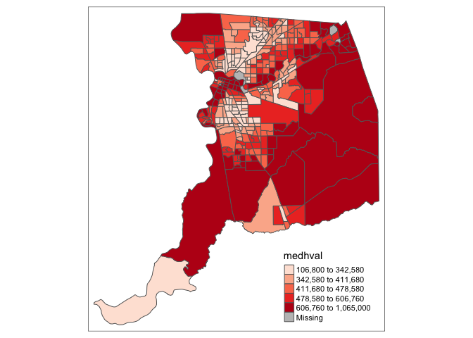
You’ve just created your first map in this class (and perhaps ever). Hooray!
tmap allows users to specify the classification
style with the fill.scale = argument. For this argument you
will need to specify the style = within
tm_scale(). The default setting uses ‘pretty’ breaks. Let’s
use style = "quantile", which tells R to break up the
shading into quantiles, or equal groups of 5.
tm_shape(sac.county.tracts) +
tm_polygons(fill = "medhval",
fill.scale = tm_scale(style = "quantile"))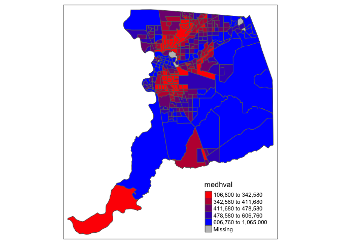
The most useful classification styles are described in the bullet points below.
style = pretty, the default setting, rounds breaks into whole numbers where possible and spaces them evenlystyle = equaldivides input values into bins of equal range, and is appropriate for variables with a uniform distribution (not recommended for variables with a skewed distribution as the resulting map may end-up having little color diversity)style = quantileensures the same number of observations fall into each category (with the potential down side that bin ranges can vary widely)style = jenksidentifies groups of similar values in the data and maximizes the differences between categoriesstyle = sddivides the values by standard deviations above and below the mean.style = catwas designed to represent categorical values and assures that each category receives a unique color
You can also manually set your own breaks using the argument
breaks = and then specifying the cutoffs within a
vector.
tm_shape(sac.county.tracts) +
tm_polygons(fill = "medhval",
fill.scale = tm_scale(breaks = c(0, 200000, 500000, 750000, 1000000)))## Warning: Values have found that are higher than the highest break. They are
## assigned to the highest interval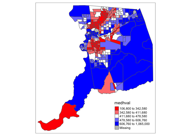
Note the message indicating that there are values larger than the
highest value specified in the breaks vector, which means the highest
(lowest) value in breaks = should match or be higher
(lower) than the maximum (minimum) value of the variable. The importance
of choosing the appropriate classification scheme is discussed in
Handout 5. You’ll get some practice trying out other classification
schemes in this week’s assignment. Note that tmap is
smart enough to detect the presence of missing values, and shades them
gray and labels them on the legend.
You can overlay multiple features on one map. For example, we can add
park polygons on top of county tracts, providing a visual association
between parks and median housing values. Here, we add another
tm_shape() and tm_polygons() to the above
code. We use the argument col = "green" to color the
polygons green.
tm_shape(sac.county.tracts) +
tm_polygons(fill = "medhval",
fill.scale = tm_scale(style = "quantile")) +
tm_shape(parks) +
tm_polygons(col = "green")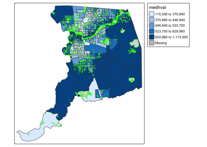
We will explore the use of tm_dots() in a future
lab.
Color Scheme
Don’t like the default blue color scheme? We can change the color
scheme using the argument values = within the
tm_scale() function. The argument values =
defines the color ranges associated with the bins as determined by the
style = argument. It expects a vector of colors or a new
color palette name.
There are three main groups of color palettes: categorical, sequential and diverging, and each of them serves a different purpose. Categorical palettes consist of easily distinguishable colors and are most appropriate for categorical data (i.e., color patch maps) without any particular order such as urban, suburban and rural, or land cover classes.
The second group is sequential palettes. These follow a gradient, for
example from light to dark colors (light colors often tend to represent
lower values), and are appropriate for continuous (numeric) variables.
Below we use the color scheme “reds” using
value = "reds".
tm_shape(sac.county.tracts) +
tm_polygons(fill = "medhval",
fill.scale = tm_scale(style = "quantile",
values = "reds"))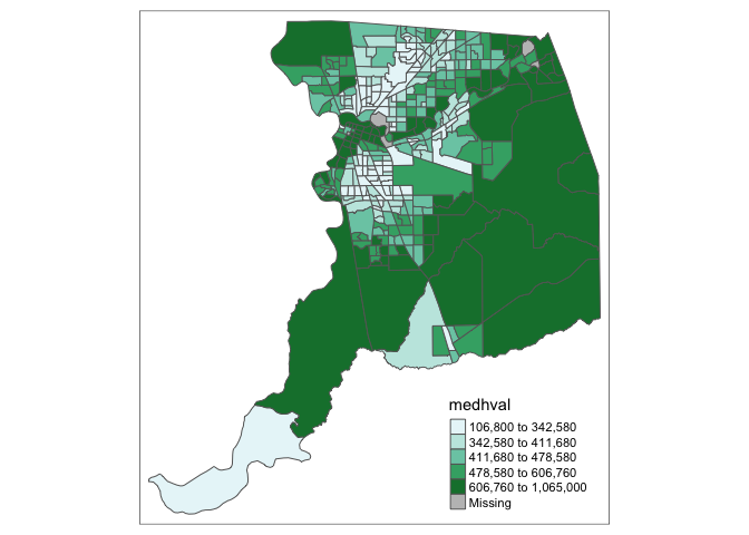
The third group, diverging palettes, typically range between three
distinct colors and are usually created by joining two single-color
sequential palettes with the darker colors at each end. Their main
purpose is to visualize the difference from an important reference
point. For instance, if we used c(“red”, “blue”), the color
spectrum would move from red to purple, then to blue, with in between
shades. In our example:
tm_shape(sac.county.tracts) +
tm_polygons(fill = "medhval",
fill.scale = tm_scale(style = "quantile",
values = c("red","blue")))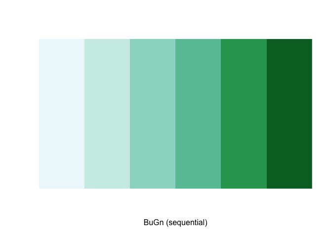
In order to capture a clearer diverging scale, we insert “white” in between red and blue.
tm_shape(sac.county.tracts) +
tm_polygons(fill = "medhval",
fill.scale = tm_scale(style = "quantile",
values = c("red","white", "blue")))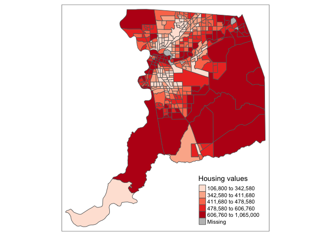
A preferred approach to select a color palette is to chose one of the
schemes contained in the RColorBrewer package. These
are based on the research of cartographer Cynthia Brewer (see the
colorbrewer2 web
site for details). RColorBrewer makes a distinction
between sequential scales (for a scale that goes from low to high),
diverging scales (to highlight how values differ from a central
tendency), and qualitative scales (for categorical variables). For each
scale, a series of single hue and multi-hue scales are suggested. In the
RColorBrewer package, these are referred to by a name
(e.g., the “Reds” palette we used above is an example). The full list is
contained in the RColorBrewer documentation.
You should have noticed from the messages produced from the mapping
above that the default “reds” palette is from
RColorBrewer. You can avoid seeing this message in the
future by specifying “brewer.reds” for values =.
There are two very useful commands in this package. One sets a color palette by specifying its name and the number of desired categories. The result is a character vector with the hex codes of the corresponding colors.
For example, we select a sequential color scheme going from blue to
green, as BuGn, by means of the command
brewer.pal, with the number of categories (5) and the
scheme as arguments. The resulting vector contains the HEX codes for the
colors.
pal <- brewer.pal(5,"BuGn")
pal## [1] "#EDF8FB" "#B2E2E2" "#66C2A4" "#2CA25F" "#006D2C"The command display.brewer.pal() allows us to view the
color scheme, and explore others, before applying them to a map. For
example:
display.brewer.pal(5,"BuGn")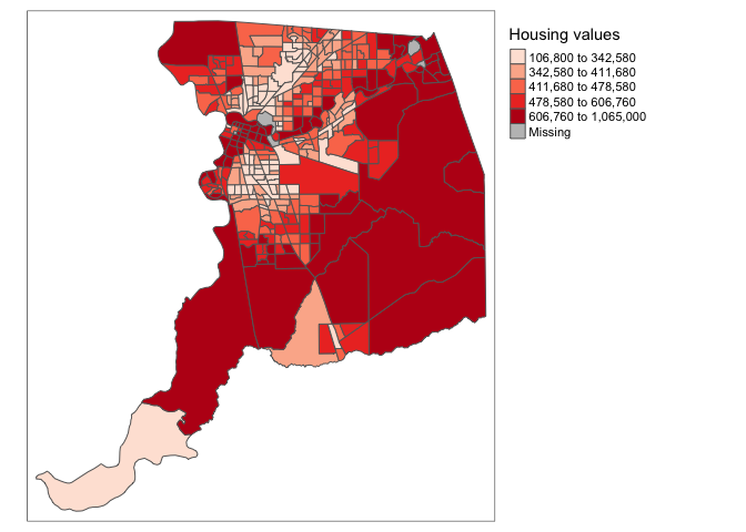
Using this palette in our map yields the following result.
tm_shape(sac.county.tracts) +
tm_polygons(fill = "medhval",
fill.scale = tm_scale(style = "quantile",
values = pal))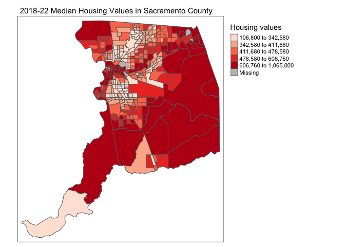
See Ch. 9.2.4 in GWR for a fuller discussion on color and other schemes you can specify.
Legend
There are many options to change the formatting of the legend. Use
the tm_legend() function within tm_polygons()
to change its title, position, orientation, or even disable it. Often,
the automatic title for the legend is not intuitive, since it is simply
the variable name (in our case, medhval). This can be
customized by setting the title = argument within the
tm_legend() function. Let’s change the legend title to
“Median housing values”
tm_shape(sac.county.tracts) +
tm_polygons(fill = "medhval",
fill.scale = tm_scale(style = "quantile",
values = "reds"),
fill.legend = tm_legend(title = "Median housing values"))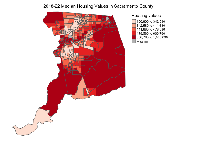
Another important aspect of the legend is its positioning. This is
handled through the position = argument within
tm_legend(). The default is to position the legend outside
of the map frame at the top right. Often, this default solution is
appropriate, but sometimes further control is needed. We can move the
legend outside or inside the mapping frame using the functions
tm_pos_out(), which keeps the legend outside of the map
frame and tm_pos_in(), which keeps it inside. Within each
of these functions, you specify two values that represent the horizontal
position (“left”, “center”, or “right”), and the vertical position
(“bottom”, “center”, or “top”). For example, to move the legend to the
bottom right in the inside of the map frame:
tm_shape(sac.county.tracts) +
tm_polygons(fill = "medhval",
fill.scale = tm_scale(style = "quantile",
values = "reds"),
fill.legend = tm_legend(title = "Median housing values",
position = tm_pos_in("right", "bottom")))
The legend is too big to fit inside the frame without obscuring some
of the map. There are a number of ways to adjust this, but one method is
to adjust the overall scale of the map. This will automatically adjust
the legend. To adjust the scale, you will need to use the argument
scale = within the function tm_layout(), which
is added after the tm_polygons() function, and allows you
to adjust the overall features of a map. The default scale is 1. When
you reduce the scale below 1, the legend shrinks relative to the size of
the map. Let’s reduce it by 0.6, or 40%.
tm_shape(sac.county.tracts) +
tm_polygons(fill = "medhval",
fill.scale = tm_scale(style = "quantile",
values = "reds"),
fill.legend = tm_legend(title = "Median housing values",
position = tm_pos_in("right", "bottom"))) +
tm_layout(scale = 0.6)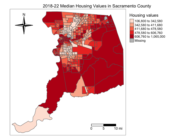
If you find the frame around the legend distracting, you can remove
it by using the argument frame = within
tm_legend() and setting it to FALSE.
tm_shape(sac.county.tracts) +
tm_polygons(fill = "medhval",
fill.scale = tm_scale(style = "quantile",
values = "reds"),
fill.legend = tm_legend(title = "Median housing values",
position = tm_pos_in("right", "bottom"),
frame = FALSE)) +
tm_layout(scale = 0.6)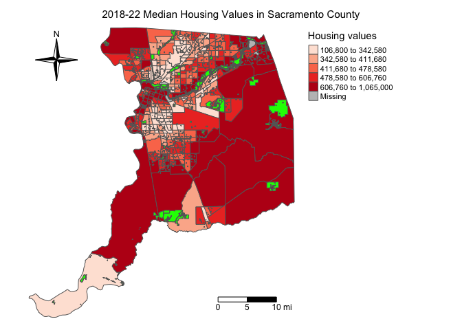
We can also customize the background color of the legend, its
alignment, font, etc. The tm_legend() function has a vast
number of options, as detailed in the documentation.
Also check Ch. 9.2.5 in GWR and the official tmap website for more examples.
Title
An important feature that you typically include in a map is the
title. We can set the title of the map using the function
tm_title(). In addition to setting the title, let’s also
move the legend back to the outside of the map frame.
tm_shape(sac.county.tracts) +
tm_polygons(fill = "medhval",
fill.scale = tm_scale(style = "quantile",
values = "reds"),
fill.legend = tm_legend(title = "Median housing values",
frame = FALSE)) +
tm_title("2019-2023 Median Housing Values in Sacramento County") +
tm_layout(scale = 0.6)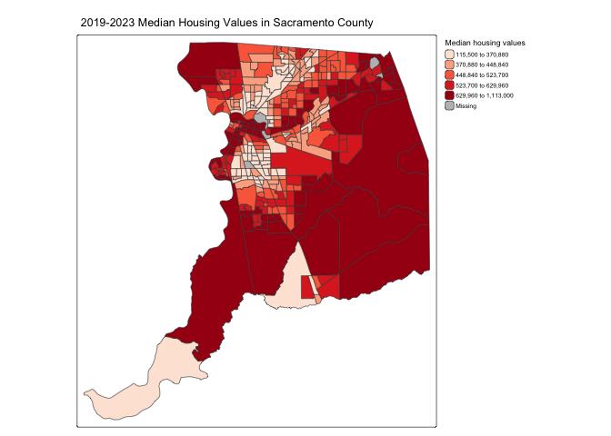
The default position of the title is at the center outside of the
frame. Similar to the legend, you can position the title using the
position = argument and the functions
tm_pos_in() and tm_pos_out(). For example, the
following code moves the the title inside the frame, and positions it
center and right:
tm_shape(sac.county.tracts) +
tm_polygons(fill = "medhval",
fill.scale = tm_scale(style = "quantile",
values = "reds"),
fill.legend = tm_legend(title = "Median housing values",
frame = FALSE)) +
tm_title("2019-2023 Median Housing Values in Sacramento County",
position = tm_pos_in("center", "top")) +
tm_layout(scale = 0.6)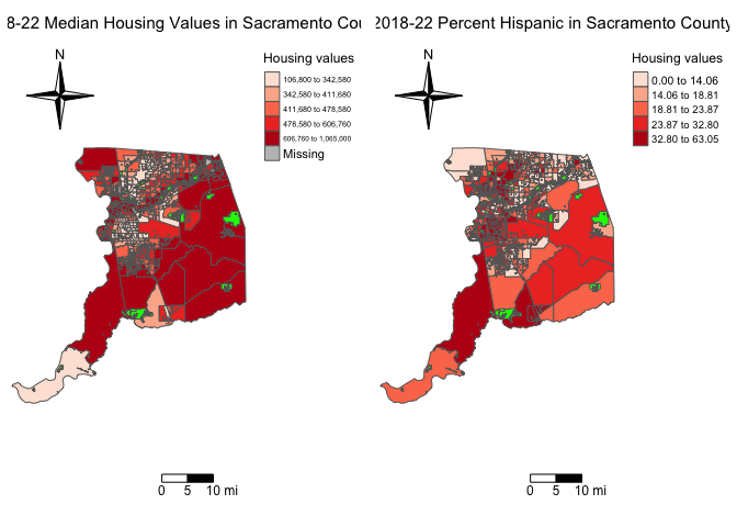
Not good, so we’ll keep it outside.
There are many arguments within tm_title() that will
allow you to change the font type, color, size and other features of the
title.
Scale bar and arrow
We need to add the other key map components described in Handout 5.
Here we add more layout functions after tm_polygons() using
the + operator. First, the scale bar, which you can add
using the function tm_scalebar(). Let’s also move the title
back to the outside of the map frame by removing the
position = argument
tm_shape(sac.county.tracts) +
tm_polygons(fill = "medhval",
fill.scale = tm_scale(style = "quantile",
values = "reds"),
fill.legend = tm_legend(title = "Median housing values",
frame = FALSE)) +
tm_title("2019-2023 Median Housing Values in Sacramento County") +
tm_scalebar() +
tm_layout(scale = 0.6)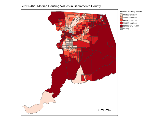
Good start, but let’s adjust a few of the features of the scale bar to make it more readable.
tm_shape(sac.county.tracts, unit = "mi") +
tm_polygons(fill = "medhval",
fill.scale = tm_scale(style = "quantile",
values = "reds"),
fill.legend = tm_legend(title = "Median housing values",
frame = FALSE)) +
tm_title("2019-2023 Median Housing Values in Sacramento County") +
tm_scalebar(breaks = c(0, 5, 10), text.size = 1,
position = tm_pos_in("right", "bottom")) +
tm_layout(scale = 0.6)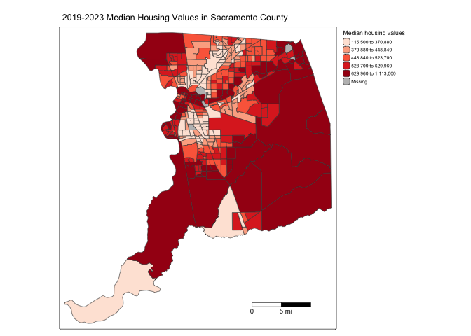
The argument breaks = within tm_scalebar()
tells R the distances to break up and end the bar. Make sure you use
reasonable break points - the Sacramento county area is not, for
example, 200 miles wide, so you should not use c(0,100,200)
(try it and see what happens. You won’t like it). Note that the scale is
in miles now (were in America!). The default is in kilometers (the rest
of the world!), but you can specify the units within
tm_shape() using the argument unit =. Here, we
used unit = "mi" to designate distance in the scale bar
measured in miles. The position = argument locates the
scale bar on the bottom right of the map. The argument
text.size = controls the size of the scale bar.
The next element is the north arrow, which we can add using the
function tm_compass(). You can control for the type, size
and location of the arrow within this function. We place a 4-star arrow
using the type = argument at the top left of the map using
the tm_pos_in() function for the position =
argument.
tm_shape(sac.county.tracts, unit = "mi") +
tm_polygons(fill = "medhval",
fill.scale = tm_scale(style = "quantile",
values = "reds"),
fill.legend = tm_legend(title = "Median housing values",
frame = FALSE)) +
tm_title("2019-2023 Median Housing Values in Sacramento County") +
tm_scalebar(breaks = c(0, 5, 10), text.size = 1,
position = tm_pos_in("right", "bottom")) +
tm_compass(type = "4star", position = tm_pos_in("left", "top")) +
tm_layout(scale = 0.6)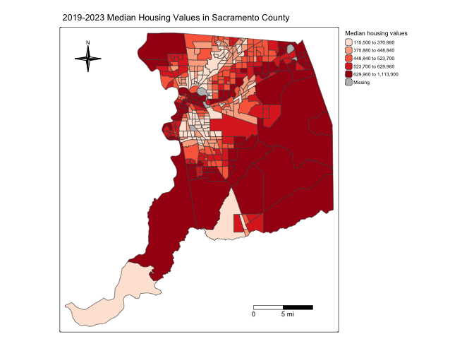
Other features
One of advantages that tmap has over other R mapping
packages is that it provides users greater ability to change a variety
of settings to make their maps prettier. For example, we can
eliminate the frame around the map using the argument
frame = FALSE within tm_layout(). Let’s also
add back the parks.
sacmhval.map <- tm_shape(sac.county.tracts, unit = "mi") +
tm_polygons(fill = "medhval",
fill.scale = tm_scale(style = "quantile",
values = "reds"),
fill.legend = tm_legend(title = "Median housing values",
frame = FALSE)) +
tm_title("2019-2023 Median Housing Values in Sacramento County") +
tm_scalebar(breaks = c(0, 5, 10), text.size = 1,
position = tm_pos_in("right", "bottom")) +
tm_compass(type = "4star", position = tm_pos_in("left", "top")) +
tm_layout(scale = 0.6, frame = FALSE) +
tm_shape(parks) +
tm_polygons(col = "green")
sacmhval.map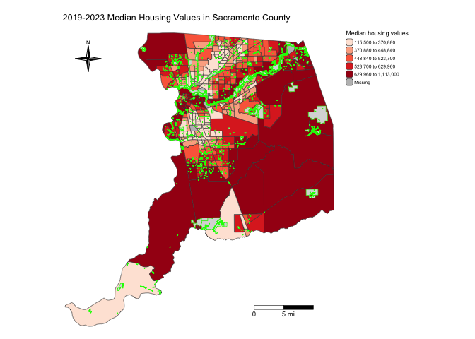
Notice that we stored the map into an object called sacmhval.map. R is an object-oriented language, so everything you make in R are objects that can be stored for future manipulation. This includes maps. You should see sacmhval.map in your Environment window. By storing the map, you can access it anytime during your current R session.
Multiple maps can be arranged in a single plot. You can do this a
couple of different ways. First, multiple maps can be defined by
specifying multiple data variable names within
tm_polygon(). For example, to show housing values and
percent Hispanic side by side, specify
fill = c("medhval", "phisp"):
tm_shape(sac.county.tracts, unit = "mi") +
tm_polygons(fill = c("medhval", "phisp"),
fill.scale = tm_scale(style = "quantile",
values = "reds"),
fill.legend = tm_legend(frame = FALSE)) +
tm_scalebar(breaks = c(0, 5, 10), text.size = 1,
position = tm_pos_in("right", "bottom")) +
tm_compass(type = "4star", position = tm_pos_in("left", "top")) +
tm_layout(scale = 0.6, frame = FALSE) +
tm_shape(parks) +
tm_polygons(col = "green")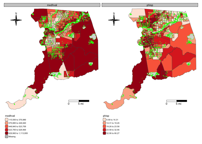
You can also use save maps into objects, and arrange them onto a plot
using the function tmap_arrange(). Let’s create the percent
Hispanic map, and save it into an object named
sacphisp.map.
sacphisp.map <- tm_shape(sac.county.tracts, unit = "mi") +
tm_polygons(fill = "phisp",
fill.scale = tm_scale(style = "quantile",
values = "reds"),
fill.legend = tm_legend(title = "% Hispanic",
frame = FALSE)) +
tm_title("2019-2023 Percent Hispanic in Sacramento County") +
tm_scalebar(breaks = c(0, 5, 10), text.size = 1,
position = tm_pos_in("right", "bottom")) +
tm_compass(type = "4star", position = tm_pos_in("left", "top")) +
tm_layout(scale = 0.6, frame = FALSE) +
tm_shape(parks) +
tm_polygons(col = "green")Then use tmap_arrange() to map sacmhval.map and
sacphisp.map side by side
tmap_arrange(sacmhval.map, sacphisp.map)
Check the full list of tm_ elements here.
Saving maps
You can save your maps a couple of ways.
- On the plotting screen where the map is shown, click on Export and save it as either an image or pdf file.
- Use the function
tmap_save()
For option 2, we can save the map object sacmhval.map as such
tmap_save(sacmhval.map,
"saccountyhval.png")Specify the tmap object and a filename with an
extension. It supports pdf, eps,
svg, wmf, png, jpg,
bmp and tiff. The default is png.
Also make sure you’ve set your directory to the folder that you want
your map to be saved in.
Interactive maps
So far we’ve created static maps. That is, maps that don’t “move”. But, we’re all likely used to Google or Bing maps - maps that we can move around and zoom into. You can make interactive maps in R using the package tmap.
To make your tmap object interactive, use the
function tmap_mode(). Type in “view” inside this
function.
tmap_mode("view")Now that the interactive mode has been ‘turned on’, all maps produced
with tm_shape() will launch. Let’s view our saved
sacmhval.map interactively.
sacmhval.map