Point Proximity Buffers
CRD 150 - Quantitative Methods in Community Research
Professor Noli Brazil
In this guide we will cover how to create and use point proximity buffers in R. Buffer analysis is used for identifying areas surrounding geographic features. The process involves generating a circle with a radius r around existing geographic features. Buffer analysis is a form of distance analysis. In this case, you connect other features based on whether they fall inside or outside the boundary of the buffer. In this guide we will extend the San Francisco Break-ins data from Lab 6. We’ll detect whether car breaks-ins tend to be clustered near certain buildings.
Setting up the data
We’ll need to load required packages. You should have already installed these packages in prior labs, so no need to run the install.packages() function.
#Load necessary packages
library(sf)
library(tidyverse)
library(tmap)We’ll then bring in four data files: (1) a shapefile of San Francisco Census tracts (2) a csv containing car breaks-in (3) a csv of San Francisco Elementary schools and (4) a list of active businesses in San Francisco. I uploaded all the files on GitHub. The code for bringing in the files and cleaning them are below. We won’t go through each line of code in detail because we’ve covered all of these operations and functions in Lab 6. We’ve embedded comments within the code briefly explaining what each chunk is doing, but go back to Lab 6 if you need further help.
#Download zip file containing San Francisco city tracts shapefile
setwd("insert your pathway here")
download.file(url = "https://raw.githubusercontent.com/crd150/data/master/sf_tracts.zip", destfile = "sf_tracts.zip")
unzip(zipfile = "sf_tracts.zip")
sf.tracts <- st_read("sf_tracts.shp")
sf.tracts.utm <- st_transform(sf.tracts, crs = "+proj=utm +zone=10 +datum=NAD83 +ellps=GRS80")#Download car-break ins.
break.df <- read_csv("https://raw.githubusercontent.com/crd150/data/master/Car_Break-ins.csv")
#Make into sf object using San Francisco tracts CRS.
break.sf <- st_as_sf(break.df, coords = c("X", "Y"), crs = st_crs(sf.tracts))
#Reproject into UTM Zone 10
break.sf.utm <- st_transform(break.sf, crs = "+proj=utm +zone=10 +datum=NAD83 +ellps=GRS80")#Download elementary schools
elem.df <- read_csv("https://raw.githubusercontent.com/crd150/data/master/elementary_schools.csv")
#Make into sf object using San Francisco tracts CRS.
elem.sf <- st_as_sf(elem.df, coords = c("longitude", "latitude"), crs = st_crs(sf.tracts))
#Reproject into UTM Zone 10
elem.sf.utm <- st_transform(elem.sf, crs = "+proj=utm +zone=10 +datum=NAD83 +ellps=GRS80")#Download businesses
bus.df <- read_csv("https://raw.githubusercontent.com/crd150/data/master/sf_businesses_2018.csv")
#Make into sf object using San Francisco tracts CRS.
bus.sf <- st_as_sf(bus.df, coords = c("lon", "lat"), crs = st_crs(sf.tracts))
#Reproject into UTM Zone 10
bus.sf.utm <- st_transform(bus.sf, crs = "+proj=utm +zone=10 +datum=NAD83 +ellps=GRS80")#Keeps car breaks-ins within San Fracisco city tract boundaries
subset.int<-st_intersects(break.sf.utm, sf.tracts.utm)
subset.int.log = lengths(subset.int) > 0
break.sf.utm <- filter(break.sf.utm, subset.int.log)
#Keeps businesses within San Fracisco city tract boundaries
subset.int<-st_intersects(bus.sf.utm, sf.tracts.utm)
subset.int.log = lengths(subset.int) > 0
bus.sf.utm <- filter(bus.sf.utm, subset.int.log)Creating buffers
The first task is to visually inspect car break-ins around elementary schools. That is, do we see clustering of points around schools? We’ll answer this question by creating buffers around schools.
The size of the buffer depends on the city you are examining and the context of your question. In this case, let’s use 150 meter buffers, which is the average size of a San Francisco city block.
We use the sf function st_buffer() to create buffers. The required arguments are your sf object and the distance.
elem.buff <-st_buffer(elem.sf.utm, 150)
elem.buff## Simple feature collection with 51 features and 15 fields
## geometry type: POLYGON
## dimension: XY
## bbox: xmin: 543716.5 ymin: 4173681 xmax: 554695.3 ymax: 4184167
## epsg (SRID): 26910
## proj4string: +proj=utm +zone=10 +ellps=GRS80 +towgs84=0,0,0,0,0,0,0 +units=m +no_defs
## # A tibble: 51 x 16
## `Campus Name` `CCSF Entity` `Lower Grade` `Upper Grade` `Grade Range`
## <chr> <chr> <int> <int> <chr>
## 1 Alamo Elemen… SFUSD 0 5 K-5
## 2 Alvarado Ele… SFUSD 0 5 K-5
## 3 Argonne Elem… SFUSD 0 5 K-5
## 4 Carver, Dr. … SFUSD 0 5 K-5
## 5 Chin, John Y… SFUSD 0 5 K-5
## 6 Chinese Educ… SFUSD 0 5 K-5
## 7 Clarendon El… SFUSD 0 5 K-5
## 8 Cleveland El… SFUSD 0 5 K-5
## 9 El Dorado El… SFUSD 0 5 K-5
## 10 Feinstein, D… SFUSD 0 5 K-5
## # ... with 41 more rows, and 11 more variables: Category <chr>, `Map
## # Label` <chr>, `Lower Age` <int>, `Upper Age` <int>, `General
## # Type` <chr>, `CDS Code` <dbl>, `Campus Address` <chr>, `Supervisor
## # District` <int>, `County FIPS` <int>, `County Name` <chr>,
## # geometry <POLYGON [m]>You’ll see that elem.buff is a polygon object like a census tract. To be clear regarding what a buffer is, let’s extract one school, El Dorado Elementary School (ID “PS028”), and its 150 meter buffer.
ex1 <- filter(elem.buff, `Map Label` == "PS028")
ex2 <- filter(elem.sf.utm, `Map Label` == "PS028")And let’s map it onto tracts with break-ins.
ex.map<-tm_shape(sf.tracts.utm) +
tm_polygons() +
tm_shape(ex1) +
tm_borders(col="red") +
tm_shape(ex2) +
tm_dots(col = "red") +
tm_shape(break.sf.utm) +
tm_dots()
tmap_mode("view")## tmap mode set to interactive viewingex.map The school we are mapping is located in the bottom right of the city. If you zoom in (Figure 1), you’ll see that the school is right in the middle of the buffer. The radius of this buffer is 150 meters, and we find that there are four break-ins located within a block of the school
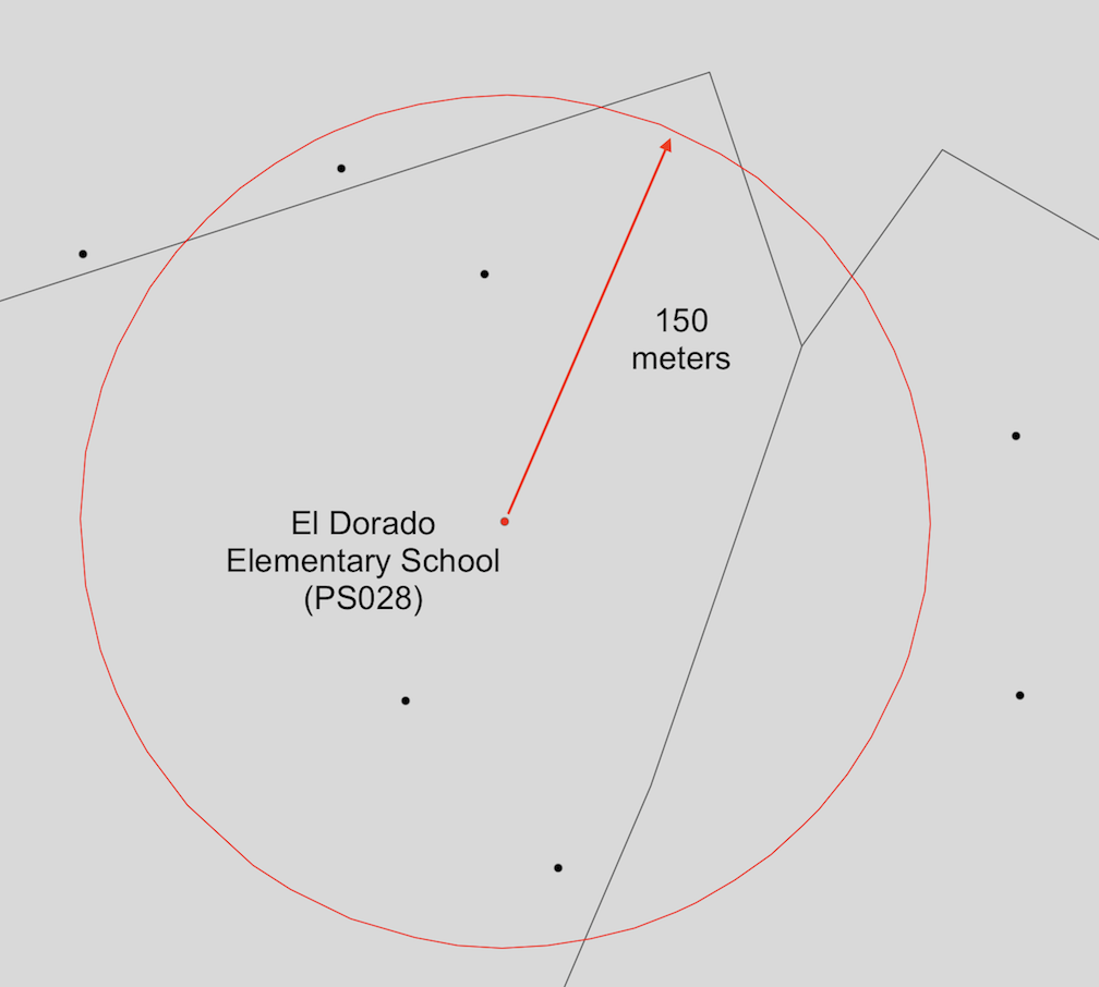
Figure 1: 150 meter buffer
One operation we can do using these buffers is to keep just the break-ins located within the buffers. We do this by using the st_intersects() function, which we went through in Lab 4.
subset.int<-st_intersects(break.sf.utm, elem.buff)
subset.int.log = lengths(subset.int) > 0
elem.buff.break <- filter(break.sf.utm, subset.int.log)The object elem.buff.break is a point sf object containing all break-ins located within 150 meters of an elementary school. One thing we can do with these data is map it.
tm_shape(sf.tracts.utm) +
tm_polygons() +
tm_shape(break.sf.utm) +
tm_dots(col = "black") +
tm_shape(elem.buff.break) +
tm_dots(col="red")