Coordinate Reference Systems
CRD 150 - Quantitative Methods in Community Research
Professor Noli Brazil
In this guide we will cover the spatial data wrangling task of converting point data from a nonspatial to a spatial format. This process involves using geographic coordinates (longitude and latitude) to place points on a map. This task is intimately related to the concept of projection and reprojection, and underlying all of these concepts is a Coordinate Reference System. In this guide, we will go through the process of using geographic coordinates to place points on a map using the San Francisco car break in data used in Lab 6.
Installing and loading packages
We’ll need to load several packages. If you have not already installed these packages, you will need to run the install.packages() function.
library(sf)
library(sp)
library(tidyverse)
library(tidycensus)
library(tigris)
options(tigris_class = "sf")
library(tmap)
library(rmapshaper)
library(tmaptools)
Longitude and Latitude
We used 2017 car break-in data in San Francisco to analyze point patterns in Lab 6. In that lab, we immediately started working on shapefile data. This guide goes back to the original csv file Car_Break-ins.csv, which contains the longitude and latitude information for each break in. We will show the steps to get from Car_Break-ins.csv to the point shapefile we used in Lab 6.
I’ve uploaded the file onto GitHub for your convenience. Use read_csv() to read it in.
break.df <- read_csv("https://raw.githubusercontent.com/crd150/data/master/Car_break_ins.csv")We will also need to bring in census tract polygon features and racial composition data using the Census API and keep tracts within San Francisco city boundaries. The code for accomplishing these tasks is below. We won’t go through each line of code in detail because we’ve covered all of these operations and functions in lab. We’ve embedded comments within the code that briefly explaining what each chunk is doing, but go back to prior guides (or RDS/GWR) if you need further help.
census_api_key("YOUR API KEY GOES HERE")# Bring in census tract data.
ca.tracts <- get_acs(geography = "tract",
year = 2016,
variables = c(tpop = "B01003_001", tpopr = "B03002_001",
nhwhite = "B03002_003", nhblk = "B03002_004",
nhasn = "B03002_006", hisp = "B03002_012"),
state = "CA",
survey = "acs5",
geometry = TRUE)
# Make the data tidy, calculate percent race/ethnicity, and keep essential vars.
ca.tracts <- ca.tracts %>%
select(-(moe)) %>%
spread(key = variable, value = estimate) %>%
mutate(pnhwhite = nhwhite/tpopr, pnhasn = nhasn/tpopr,
pnhblk = nhblk/tpopr, phisp = hisp/tpopr) %>%
select(c(GEOID,tpop, pnhwhite, pnhasn, pnhblk, phisp))
# Bring in city boundary data
pl <- places(state = "CA", cb = TRUE)
# Keep SF city
sf.city <- filter(pl, NAME == "San Francisco")
# Keep tracts that intersect SF city boundary.
# Eliminate Farallon and Treasure Islands
sf.tracts <- ms_clip(ca.tracts, sf.city, remove_slivers = TRUE) %>%
filter(GEOID != "06075980401" & GEOID != "06075017902")Converting point coordinates
The object break.df is just a basic tibble (data frame), not a spatial sf points object. To convert these data into spatial points, we’ll need to “locate” them onto a map. Luckily, our data have longitude (x-coordinate) and latitude (y-coordinate) information, where longitude is your X coordinate and spans East/West and latitude is your Y coordinate and spans North/South, so we already know where the points are located on Earth, and it’s just a matter of placing them there.
We will use the function st_as_sf() to create a point sf object out of break.df.
break.sf <- st_as_sf(break.df, coords = c("X", "Y"), crs ="+proj=longlat +datum=NAD83 +ellps=GRS80")The argument coords = specifies the (X,Y) coordinates - or longitude, latitude - of each point. In the dataframe break.df, these variables are conveniently named X and Y and are specified in st_as_sf() using the coords argument as coords = c("X", "Y").
The argument crs = specifies the Coordinate Reference System (CRS). The CRS refers to the way in which spatial data that represent the earth’s surface (which is round and 3 dimensional) are flattened so that you can “Draw” them on a 2-dimensional surface. This concept is so important, it needs to have its own section.
Coordinate Reference System
We won’t go through the real nuts and bolts of CRS, which you can read in Geocomputation with R (GWR) Chapter 2.4 and 6, but we’ll go through enough of it so that you can get through most CRS related spatial data wrangling tasks.
The CRS contains two major components: the Geographic Coordinate System (GCS) and the Projected Coordinate System (PCS). The GCS can be further separated into two parts: the ellipse and the datum. The ellipse is a model of the Earth’s shape. The datum defines the coordinate system of this model - the origin point and the axes. You need these two basic components to place points on Earth’s three-dimensional surface. Think of it as trying to create a globe (ellipse) and figuring out where to place points on that globe (datum).
The PCS then translates these points from a globe onto a two-dimensional space. We need to do this because were creating flat paper or on-the-screen maps, not globes (it’s kind of hard carrying a globe around when you’re finding your way around a city).
You can call up the CRS of a spatial data set by using the function st_crs(). For example, the CRS of the census tract data is
st_crs(break.sf)## Coordinate Reference System:
## EPSG: 4269
## proj4string: "+proj=longlat +ellps=GRS80 +towgs84=0,0,0,0,0,0,0 +no_defs"You see two ways to describe the CRS: an epsg code and a proj4string. The epsg is a shortcut way for defining all the components of a CRS in one number. You can look up all the possible epsg here.
In contrast, proj4string spells everything out. The Projected Coordinate System or PCS is defined by +proj=, in this case longlat because we have X,Y or Longitude/Latitude coordinates. How did I know what datum and ellipse to specify? Magic. Actually, there are a set of commonly used CRS datums/ellipse, which NAD83/GRS80 is one of. Check the handout in the Week 6 folder on Canvas for other common combinations.
There are three important things you should come away with from this discussion about CRS. First, as described above, the CRS has two components, the GCS and the PCS, which you need to always specify. This means that if you are bringing in spatial data, you should know what the GCS and PCS are. For example, the website you downloaded the data tells you. Or the person giving you the data tells you. Maybe a magical fairy whispered it in your ear. Whatever, you just need to know. If you specify the wrong CRS, you will encounter some problems. Any data that are in (X,Y) form has a longitude/latitude projected coordinate system. In this case, just specify the CRS we used in the code above and you should be fine.
Second, all spatial data in your current R session should have the same CRS. If they don’t, you won’t be able to overlay the objects on a map or conduct any of the multiple layer spatial operations we went through in Lab 5. We can check the CRS by using the function st_crs(). Let’s check to see if sf.tracts and break.sf have the same CRS
st_crs(sf.tracts)## Coordinate Reference System:
## EPSG: 4269
## proj4string: "+proj=longlat +ellps=GRS80 +towgs84=0,0,0,0,0,0,0 +no_defs"st_crs(break.sf)## Coordinate Reference System:
## EPSG: 4269
## proj4string: "+proj=longlat +ellps=GRS80 +towgs84=0,0,0,0,0,0,0 +no_defs"They look the same, but…
st_crs(break.sf) == st_crs(sf.tracts)## [1] TRUEYes!
Reprojecting points
The third important thing is your CRS should be compatible with the functions you plan to use on your data. An important compatibility issue is that your spatial data should have the appropriate distance metric like meters or miles. Distance in longitude/latitude is in decimal degrees which (1) most people don’t understand and (2) is not compatible with several spatial functions.
We can find out the units of a spatial data set by using the st_crs() function and calling up units as follows
st_crs(break.sf)$units## NULLst_crs(sf.tracts)$units## NULLNot good.
Let’s reproject the CRS to something that takes on meters. A popular meter-based Projected Coordinate System is Universal Tranverse Mercator (UTM). UTM separates the United States in separate zones and Northern California is in zone 10, as shown in the figure below.
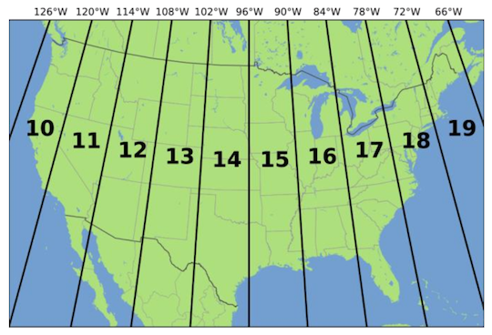
Figure 1: UTM Zones
Let’s reproject both sf.tracts and breaks.sf to a UTM Zone 10 projected coordinate system. Use +proj=utm as the PCS, NAD83 as the datum and GRS80 as the ellipse (popular choices for the projection/datum/ellipse of the U.S.). Whenever you use UTM, you also need to specify the zone, which we do by using +zone=10. To reproject use the function st_transform() as follows
sf.tracts.utm <- st_transform(sf.tracts, crs = "+proj=utm +zone=10 +datum=NAD83 +ellps=GRS80")
break.sf.utm <- st_transform(break.sf, crs = "+proj=utm +zone=10 +datum=NAD83 +ellps=GRS80")
Equal?
st_crs(sf.tracts.utm) == st_crs(break.sf.utm)## [1] TRUEUnits?
st_crs(sf.tracts.utm)$units## [1] "m"st_crs(break.sf.utm)$units## [1] "m"“m” stands for meters. Great. Now, let’s map the break ins.
tm_shape(sf.tracts.utm) +
  tm_polygons() +
tm_shape(break.sf.utm) +
  tm_dots(col="red")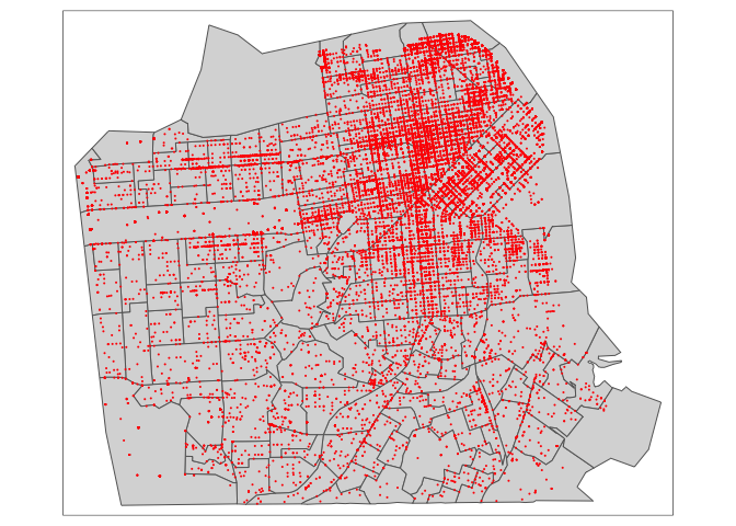
Neat.
Another important problem that you may encounter is that a shapefile or any spatial data set you downloaded from a source contains no CRS (unprojected or unknown). In this case, use the function st_set_crs() to set the CRS. See GWR 6.1 for more details.
Main takeaway points:
- The CRS for any spatial data set you bring into R should always be established.
- If you are planning to work with multiple spatial data sets on the same project, make sure they have the same CRS.
- Make sure the CRS is appropriate for the types of spatial analyses you are planning to conduct.
If you stick with these principles, you should be able to get through most issues regarding CRSs. If you get stuck, read GWR Ch. 2.4 and 6.

This work is licensed under a Creative Commons Attribution-NonCommercial 4.0 International License.
Website created and maintained by Noli Brazil